Unified Commerce Analytics
A Microsoft Fabric medallion build that turns a five-join transactional database into a Direct Lake star schema an executive can open at eight in the morning.
North Meridian Retail Group runs its point-of-sale off a heavily normalised Azure SQL database, which is exactly what a transactional system should be and exactly wrong for reporting. Getting a basic revenue number out of it meant five-plus joins across atomic tables, and the region a customer belonged to lived in a CSV on one analyst’s desktop. The brief was a Fabric Lakehouse that gets analytics off that production database entirely, without ever touching the till.
The problem
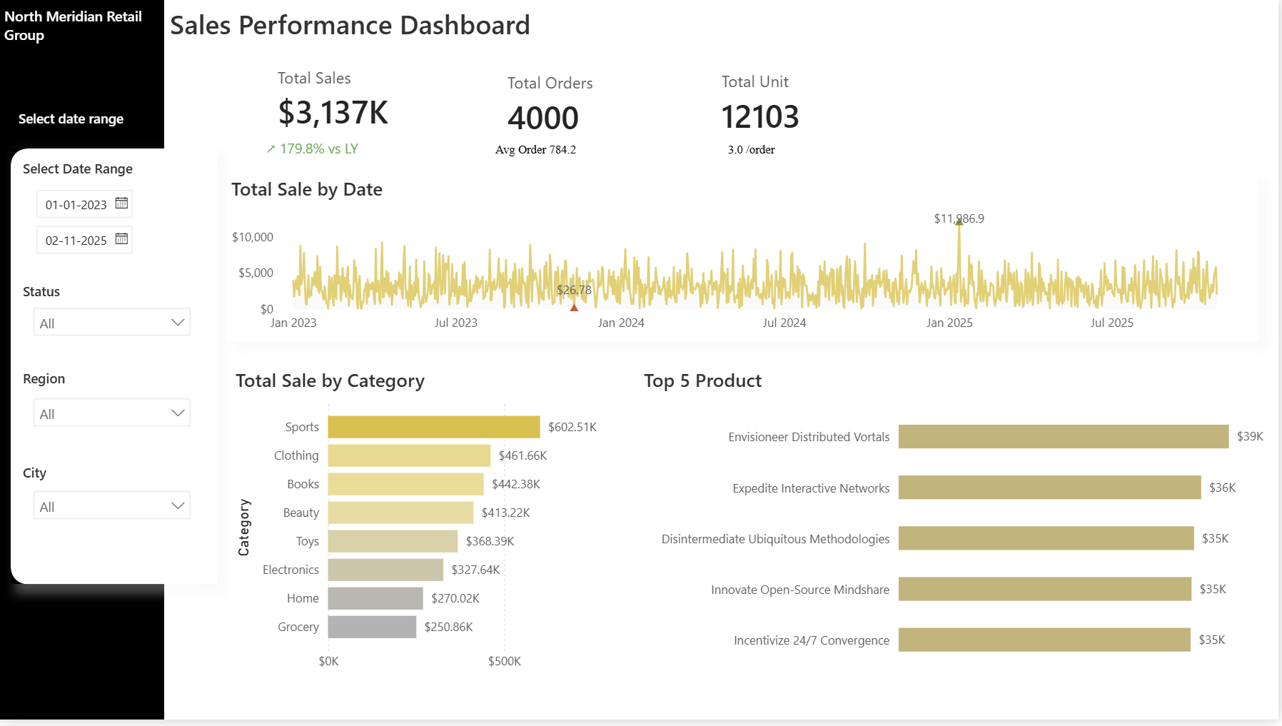
The analytics team was spending eighty percent of its week hand-writing SQL joins across Sales, Orders, Products and Customers, leaving twenty percent for actual insight work. The regional hierarchy analysts needed for reporting wasn’t in the database at all, it was RegionMapping.csv, maintained by hand, with enough drifted copies in circulation that different regions reported conflicting numbers depending on which file they’d used. North Meridian’s Head of Sales put the frustration plainly: “I do not care about Third Normal Form. I care about what my top ten products are right now.”
The fix couldn’t touch the operational database. Point-of-sale writes had to stay exactly as reliable as they were, which meant analytics needed to become a fully decoupled, read-only consumer of a governed copy of the data, not a second workload competing for the same tables.
The architecture
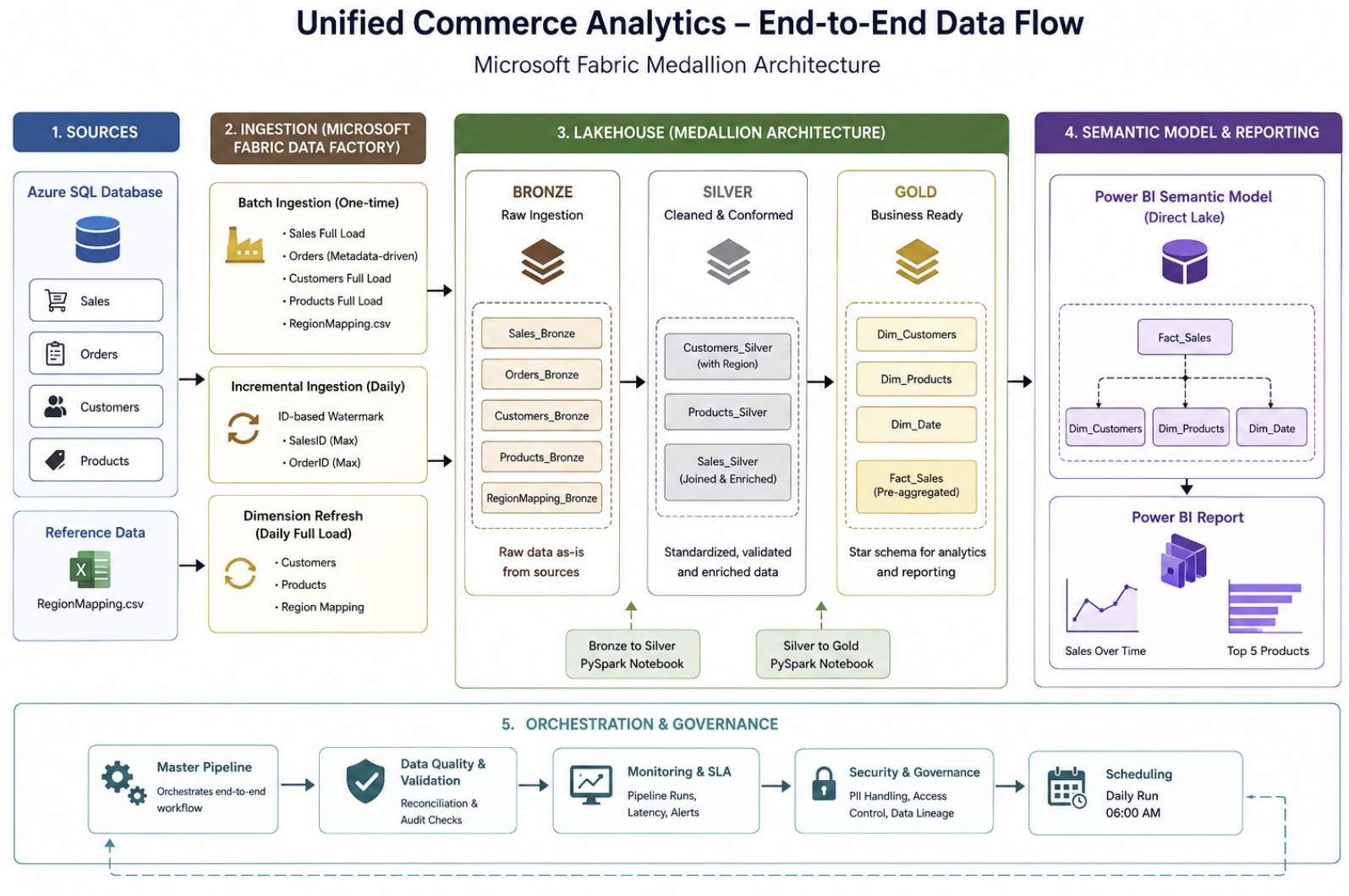
A Bronze, Silver, Gold Lakehouse, built with the same principle behind every case study in this series: each layer protects a different stakeholder. Bronze captures the four Azure SQL tables and the RegionMapping CSV exactly as they arrive, so any transformation bug downstream can be replayed from source rather than patched over. Silver joins and standardises, deriving FullName, rounding prices, denormalising region into the customer record. Gold collapses individual transactions into a pre-aggregated star schema, three dimensions and one fact table, sized for Power BI’s in-memory engine rather than for a transaction log.
 View full size (opens in a new tab)
 View full size (opens in a new tab)
 View full size (opens in a new tab)
Bronze: land everything as-is, then make reruns safe
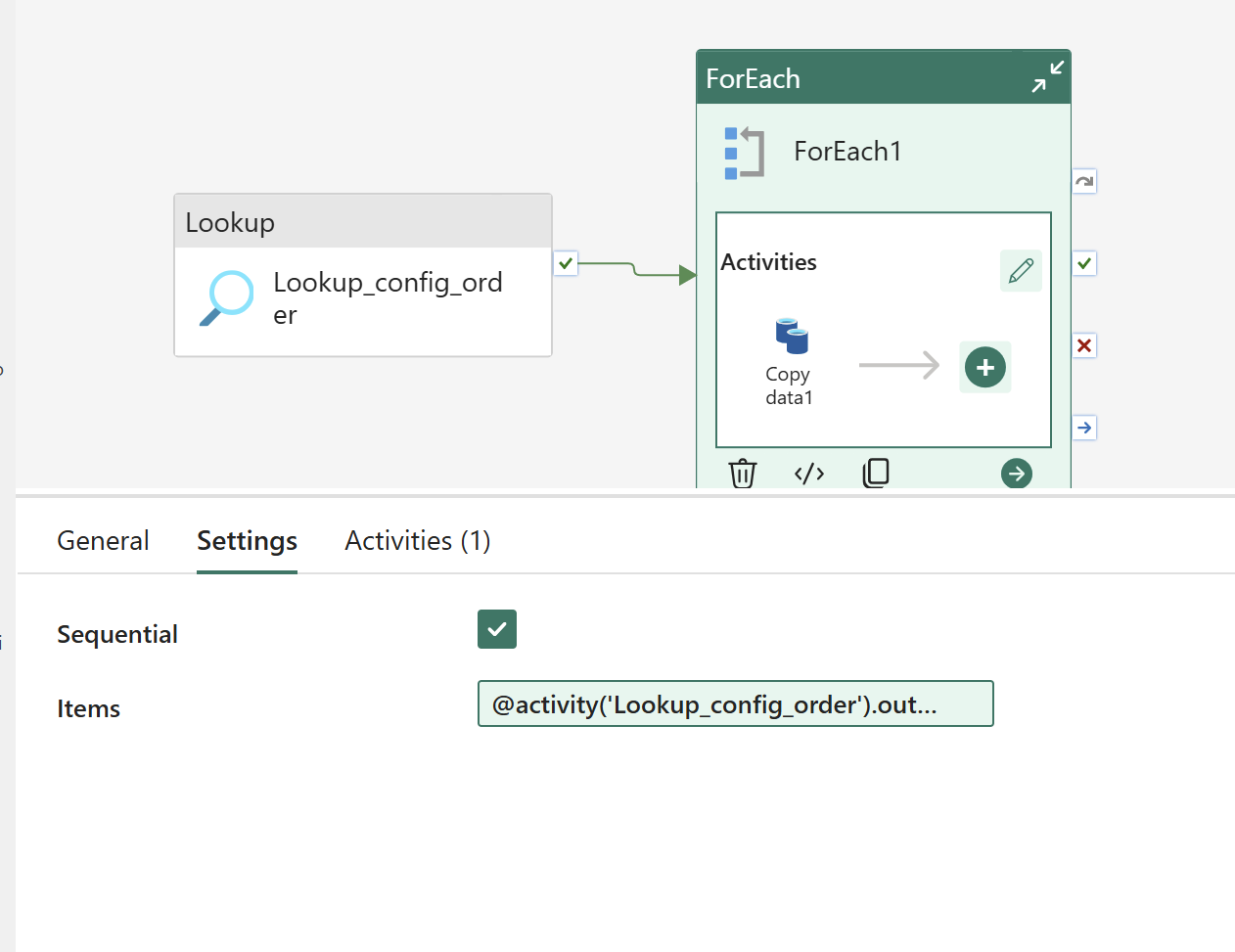
Two of the four source tables are large enough that a single unbounded Copy activity is the wrong tool. Orders gets a metadata-driven pattern instead: a control table holding OrderID ranges, a Lookup activity that reads the active ranges, and a ForEach loop that fires one Copy per range.
 View full size (opens in a new tab)
Make a failed batch resumable, not restart-from-zero
Orders is too large to copy in one unbounded query, and a single monolithic Copy activity that fails partway through leaves no way to know which rows made it across without a full reload. The pipeline needs to isolate failure to one slice of the table, and let that one slice be rerun without touching the rest.
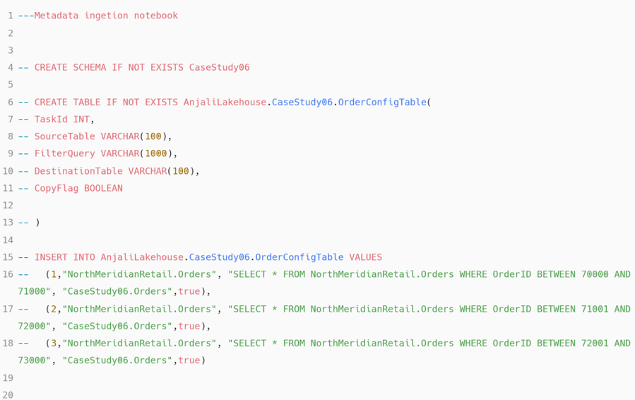
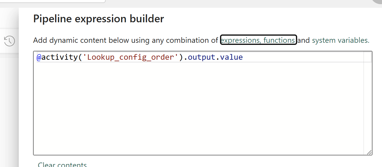
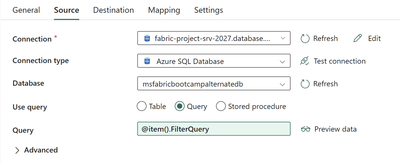
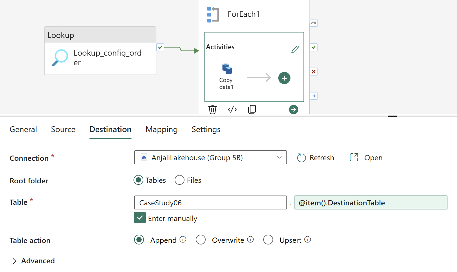
OrderConfigTable holds one row per OrderID range, each with a FilterQuery, a DestinationTable, and a CopyFlag. A Lookup activity reads the active rows, and a ForEach loop fires one Copy per row, with the source query and destination table both resolved dynamically from that row rather than hardcoded per activity.
 View full size (opens in a new tab)
 View full size (opens in a new tab)
 View full size (opens in a new tab)
 View full size (opens in a new tab)
That’s the operational payoff: a range that fails halfway through gets its CopyFlag addressed on its own, and a rerun of the pipeline picks up exactly that range, not the two that already succeeded. A single big Copy activity can’t offer that, because a partial failure inside one unbounded query gives you no row-level boundary to resume from.
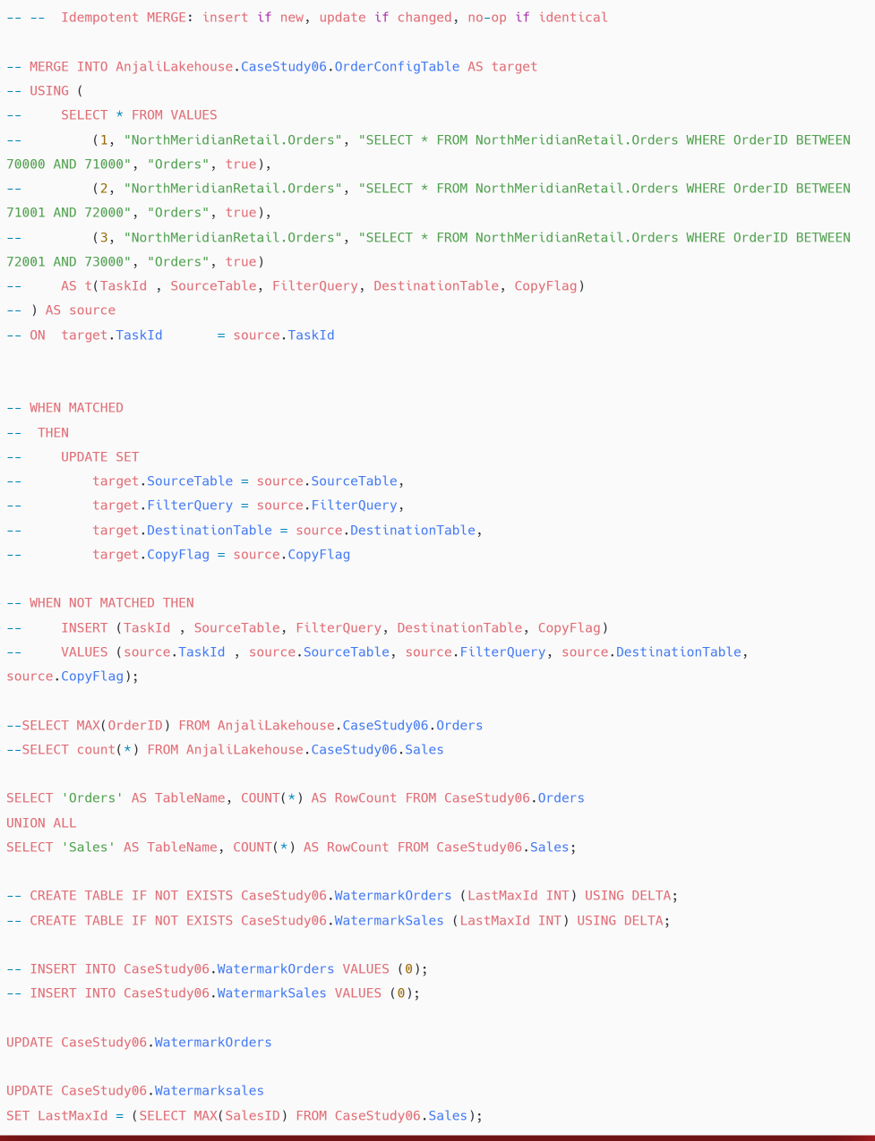
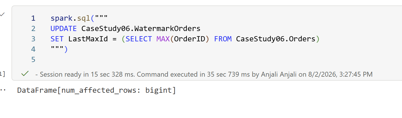
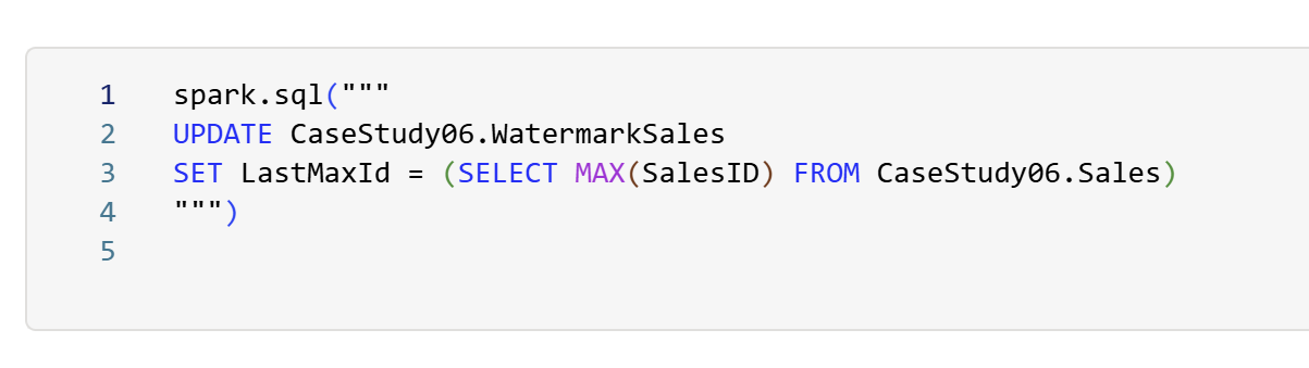
The watermark tables that make the daily incremental loads possible get seeded the same way, via commented-out scaffolding kept as a record of the one-time setup, with the live logic below it updating each watermark from the newly landed Bronze data.
 View full size (opens in a new tab)
 View full size (opens in a new tab)
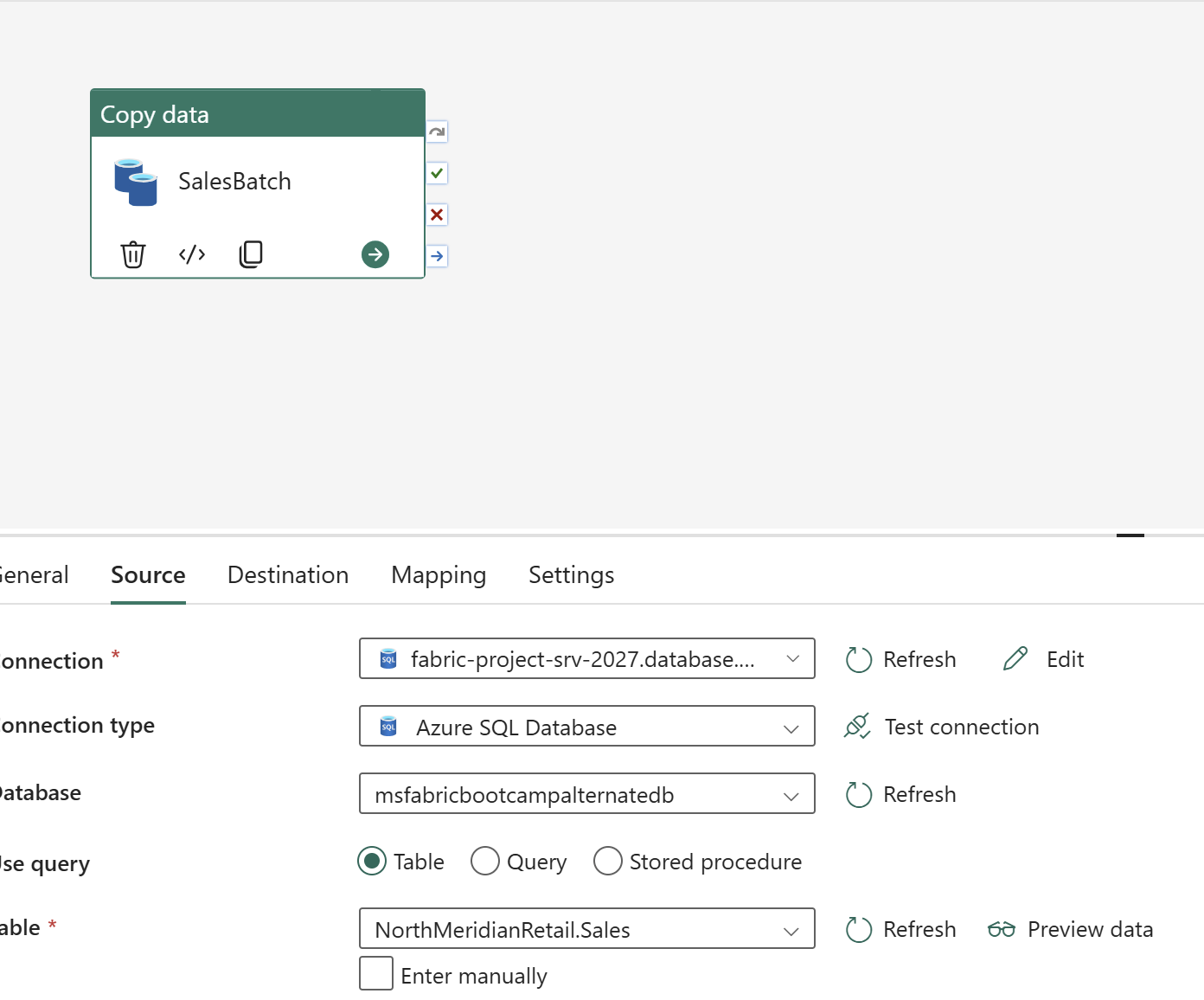
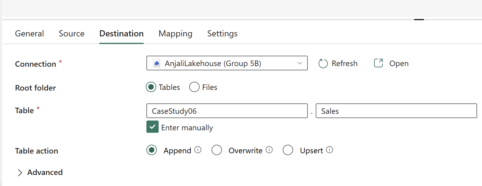
Pipeline 1 handles Sales the simple way, a single Copy activity, since a full initial load of one table doesn’t need the range-slicing machinery Orders does.
 View full size (opens in a new tab)
 View full size (opens in a new tab)
 View full size (opens in a new tab)
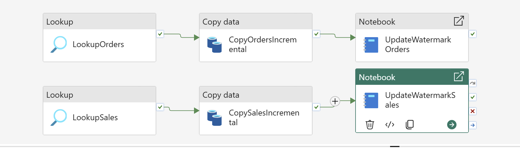
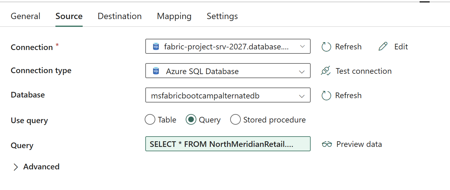
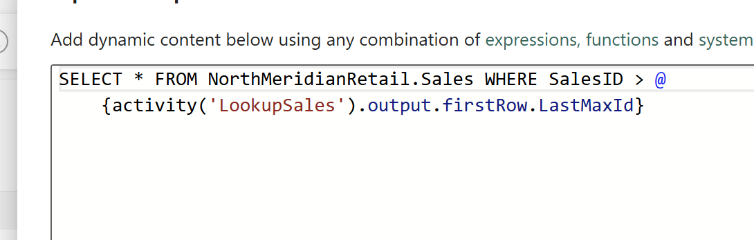
From here, the daily pipeline takes over. Pipeline 3 reads both watermark tables, pulls only the rows with a higher ID than what’s already landed, and updates the watermark again once the copy succeeds.
 View full size (opens in a new tab)
 View full size (opens in a new tab)
![Full query text: SELECT * FROM NorthMeridianRetail.Orders WHERE OrderID > @{activity('LookupOrders').output.value[0].LastMaxId}.](/_astro/pipeline3-orders-watermark-filter.CNPpmIxX.png) View full size (opens in a new tab)
View full size (opens in a new tab)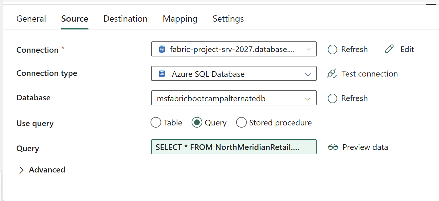 View full size (opens in a new tab)
 View full size (opens in a new tab)
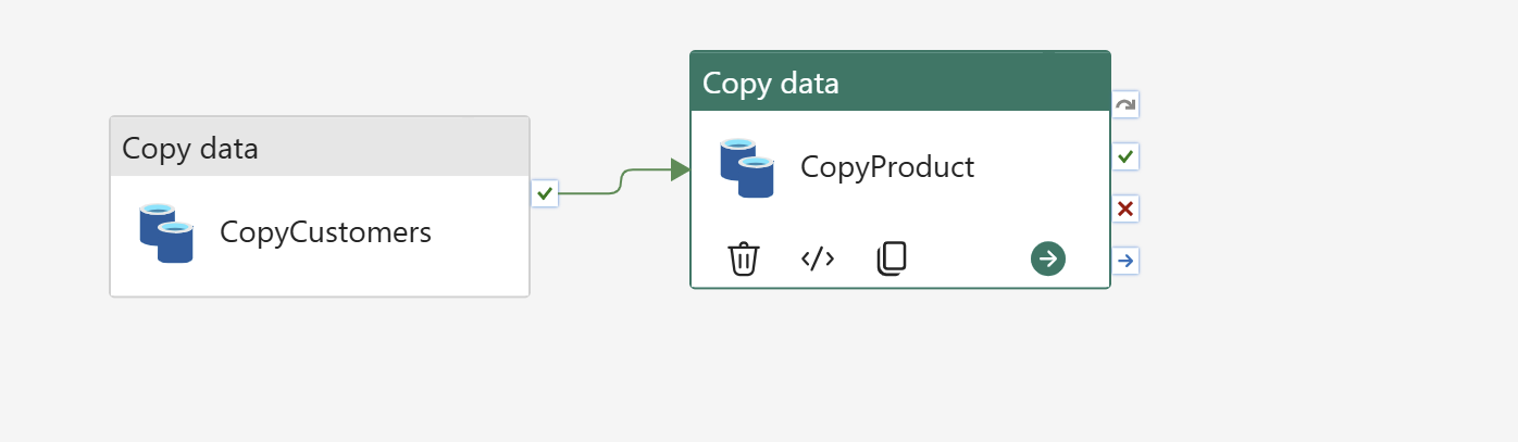
Customers and Products are small enough that daily full-refresh is simpler than tracking a watermark for them, so Pipeline 4 just re-copies both in full every run.
 View full size (opens in a new tab)
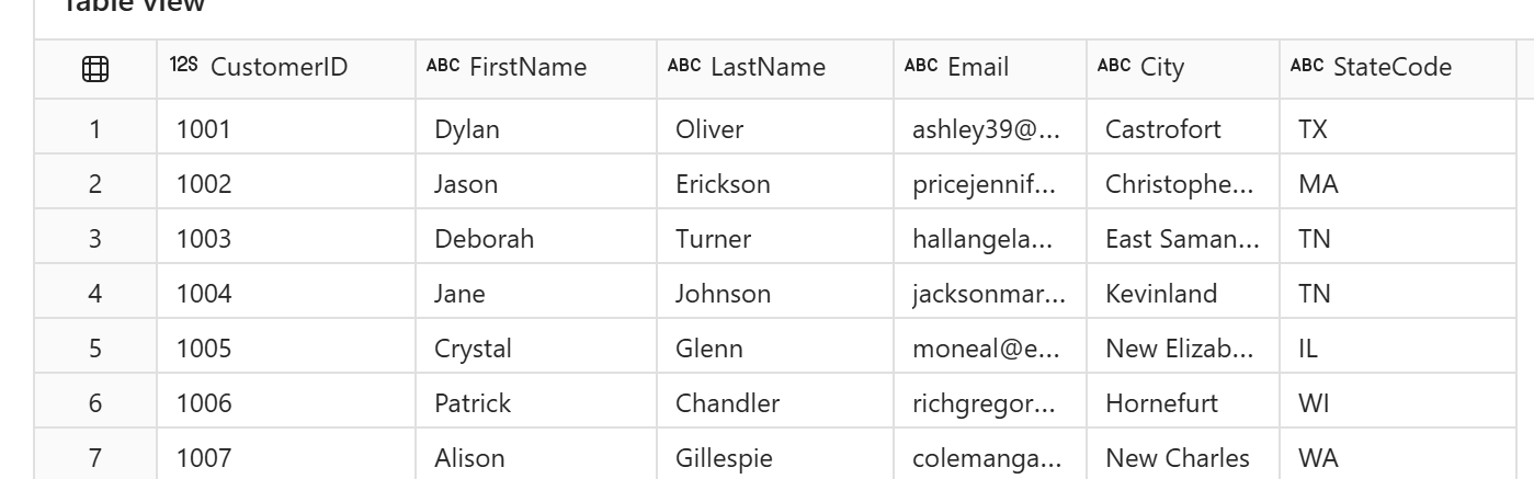
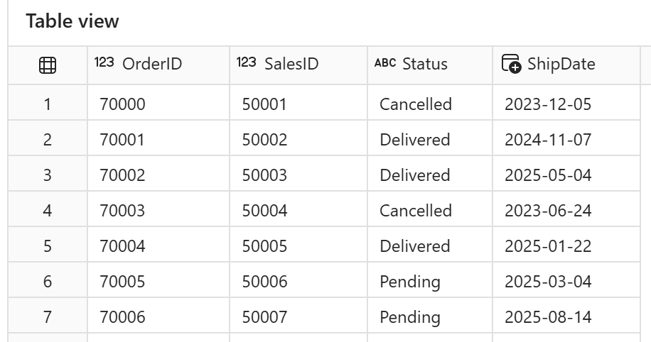
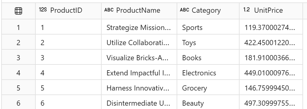
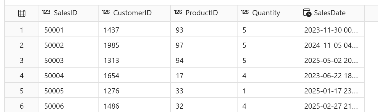
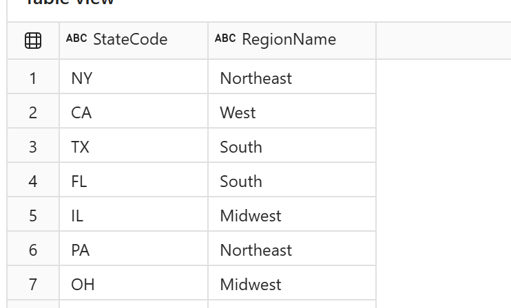
By the time the initial loads and the first incremental run have both landed, Bronze holds five governed datasets, four from Azure SQL and the region CSV, none of them transformed yet.
 View full size (opens in a new tab)
 View full size (opens in a new tab)
 View full size (opens in a new tab)
 View full size (opens in a new tab)
 View full size (opens in a new tab)
Silver: join, standardise, and denormalise region
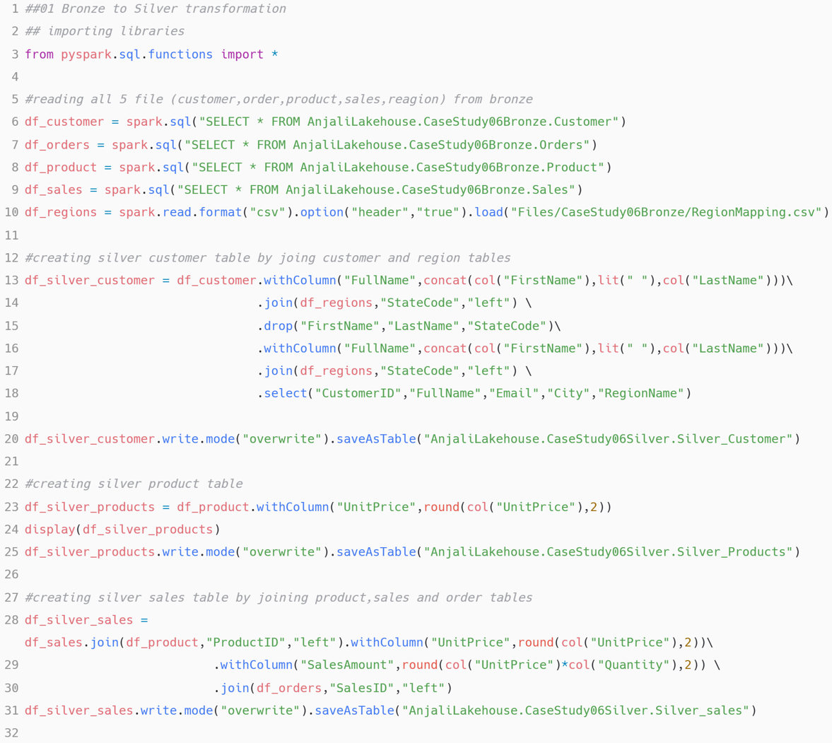
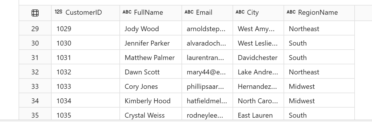
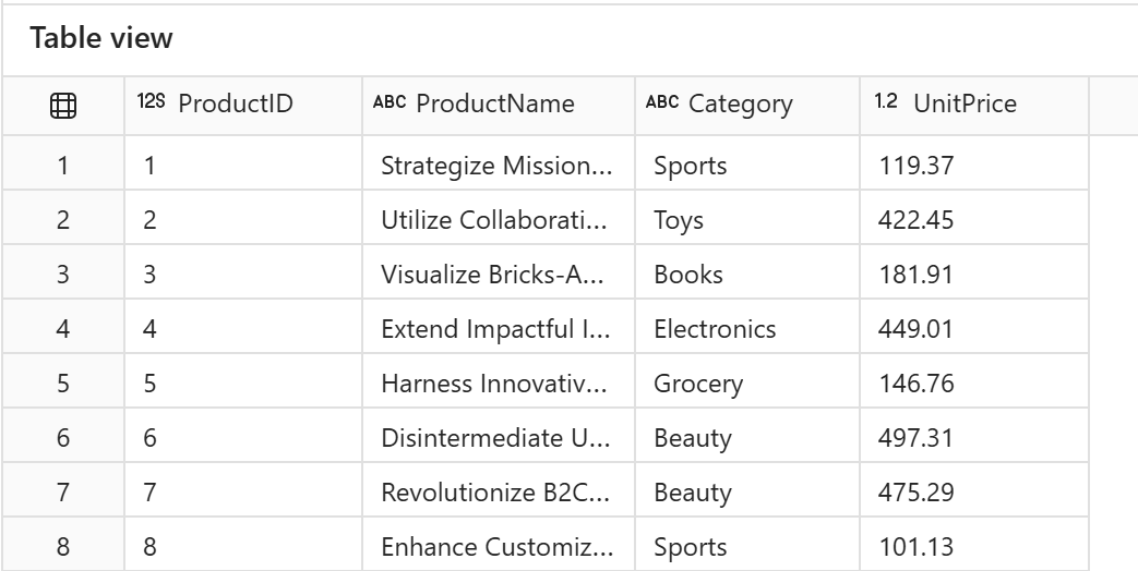
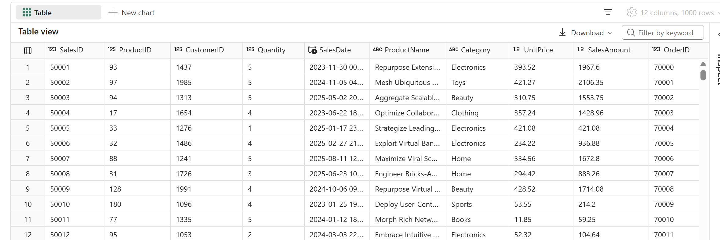
One PySpark notebook produces all three Silver tables: Customers joined to the region mapping with a derived FullName, Products with UnitPrice rounded to two decimal places, and Sales joined to both Orders and Products with a computed SalesAmount.
 View full size (opens in a new tab)
 View full size (opens in a new tab)
 View full size (opens in a new tab)
 View full size (opens in a new tab)
Gold: collapse into a star schema
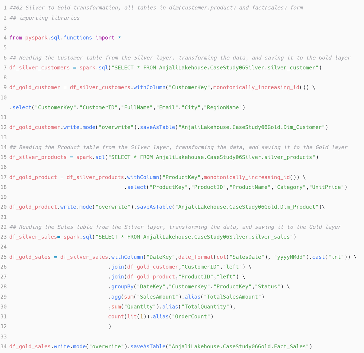
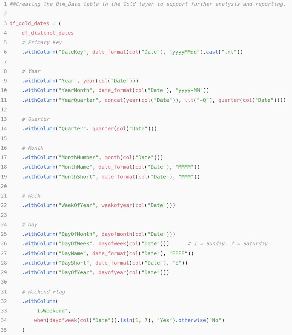
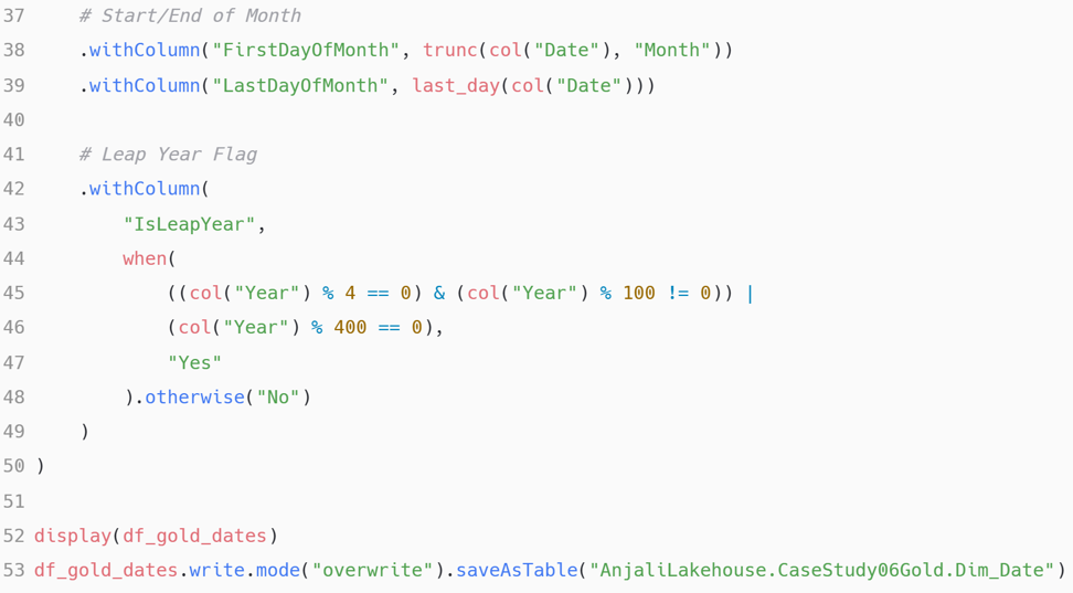
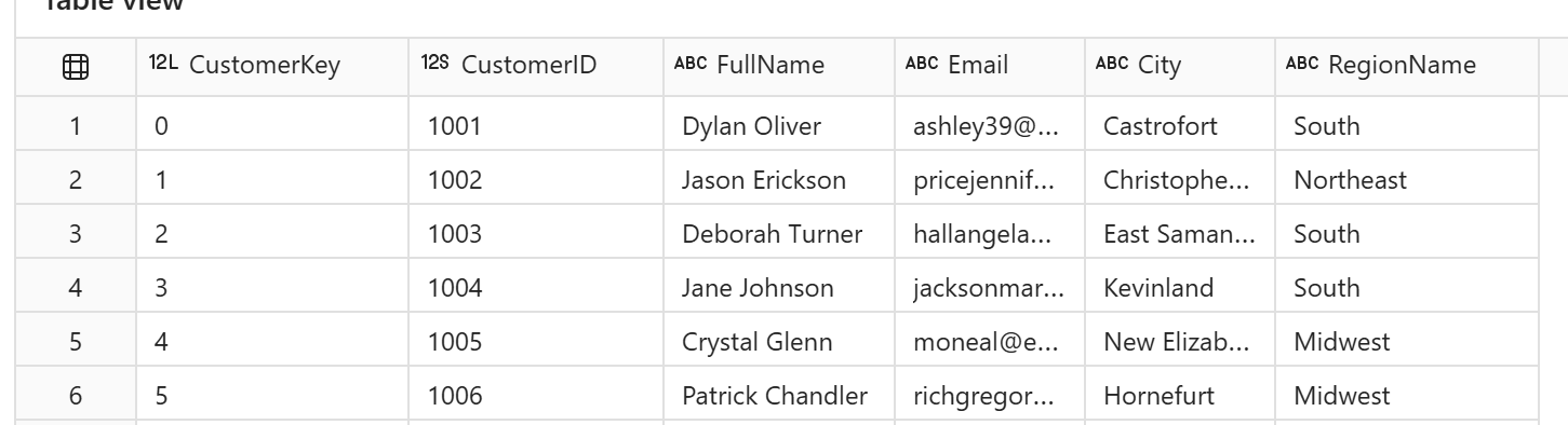
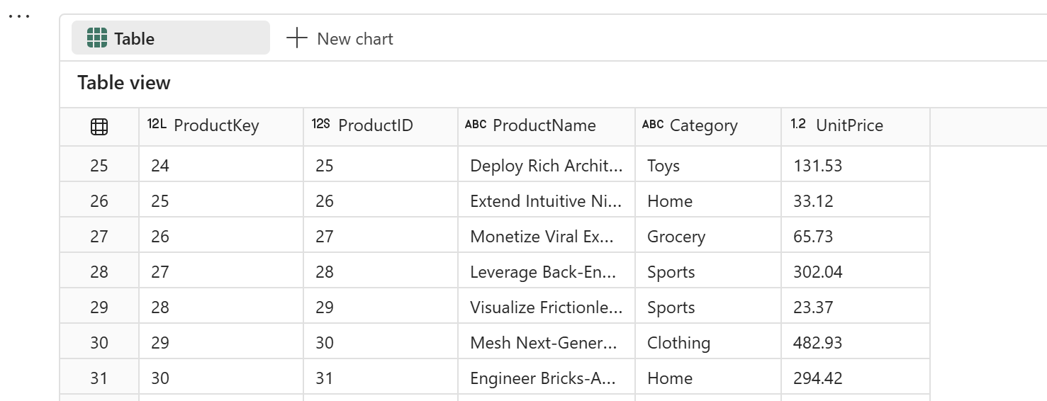
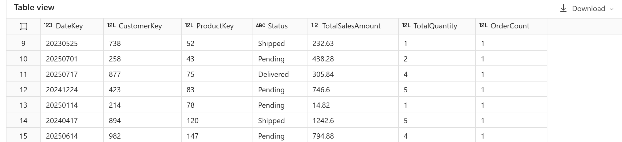
The Silver-to-Gold notebook generates surrogate keys with monotonically_increasing_id(), builds Dim_Date from the distinct dates in the data, and groups Sales down to the (DateKey, CustomerKey, ProductKey, Status) grain the brief specified.
 View full size (opens in a new tab)
 View full size (opens in a new tab)
 View full size (opens in a new tab)
 View full size (opens in a new tab)
 View full size (opens in a new tab)
 View full size (opens in a new tab)
 View full size (opens in a new tab)
The semantic model and report
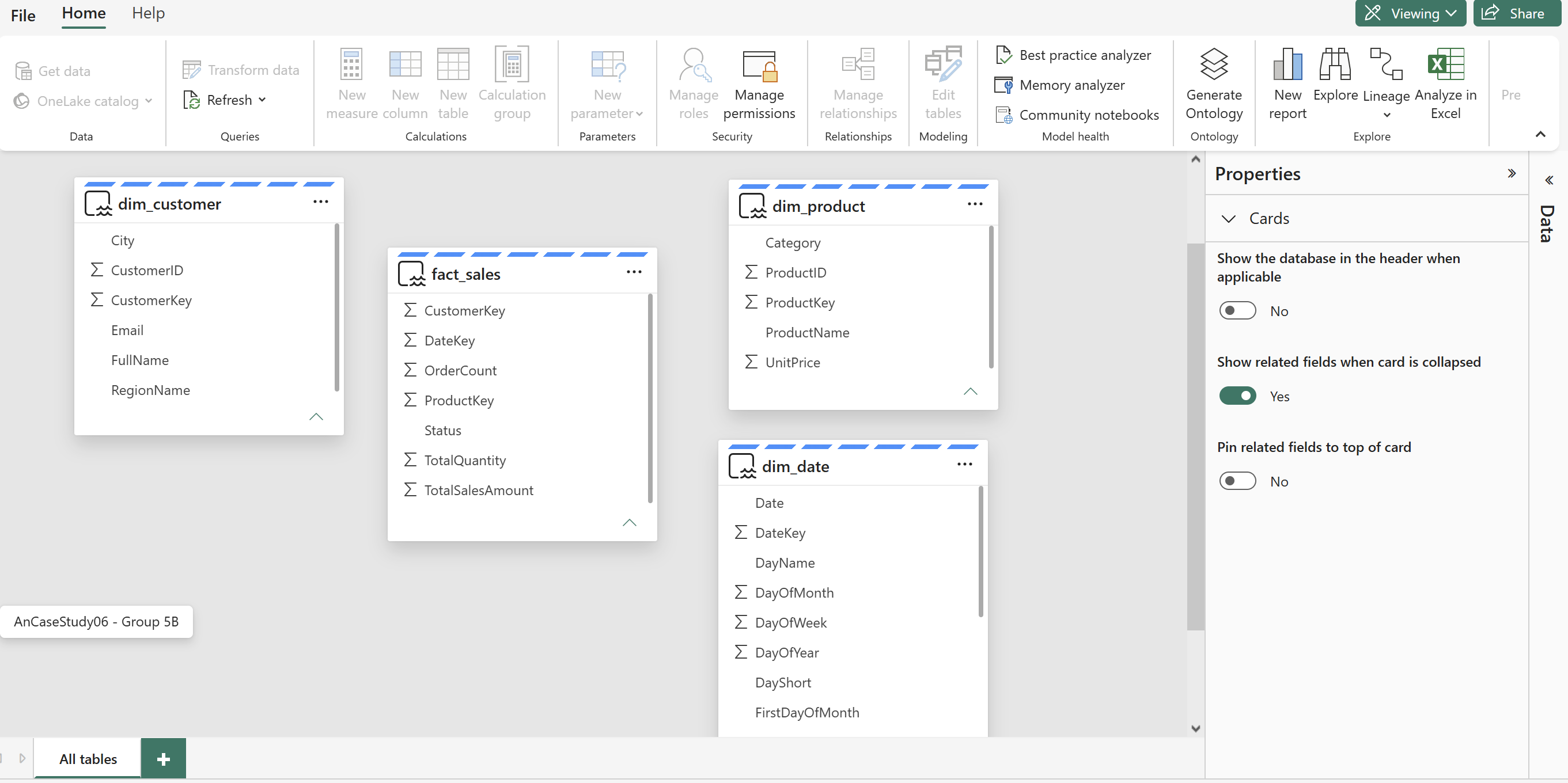
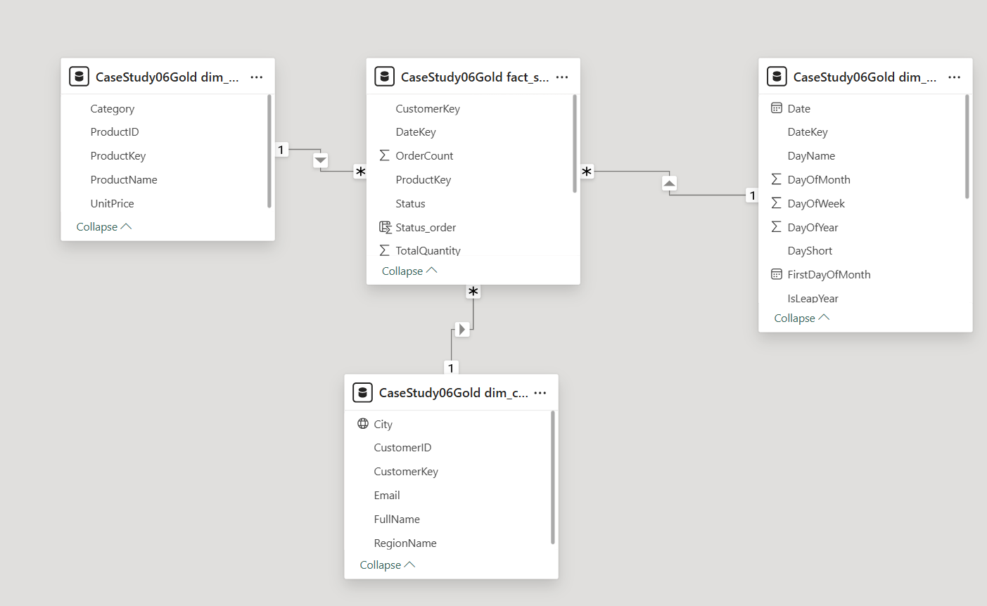
The Power BI Semantic Model connects to Gold via Direct Lake, reading the Delta tables directly rather than importing a copy, with one-to-many relationships from each dimension into Fact_Sales.
 View full size (opens in a new tab)
 View full size (opens in a new tab)
 View full size (opens in a new tab)
Orchestration
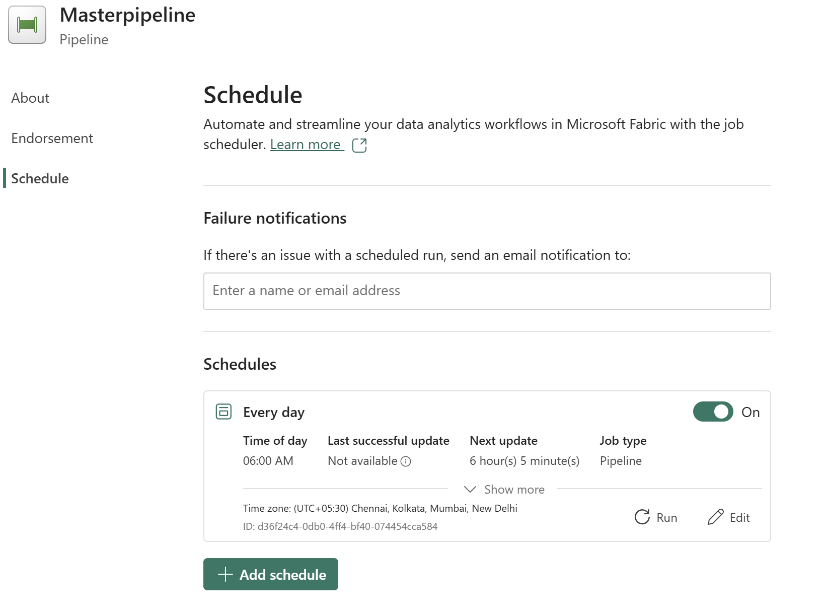
A Master Pipeline chains the daily steps in dependency order, incremental load first, then dimension refresh, then the two PySpark notebooks, then a semantic model refresh so the report never shows stale Gold data next to a fresh Bronze load.
 View full size (opens in a new tab)
 View full size (opens in a new tab)
What this proves
A five-way-join transactional database and a star schema an executive can read at 8am aren’t reconciled by picking one over the other, they’re reconciled by putting a Lakehouse between them and letting each layer do one job. Bronze makes replay possible. Silver makes the RegionMapping CSV’s version drift someone else’s problem, permanently. Gold makes the fact table small enough that Direct Lake and VertiPaq can do their job. None of that required touching the point-of-sale database once.