Databricks
PySpark

Building the Platform

A Databricks exercise in shared functions and Delta time travel, turning a hand-run notebook into a platform the next engineer can rerun without asking how.

Role: Independent case study
Year: 2026
Stack: Databricks · PySpark · Delta Lake · Delta Time Travel · Databricks Jobs

SantéFlux is a Paris health service that turns hospital and pharmacy extracts into regional analytics for care providers across France. Every report was a notebook someone ran by hand, with the same three derivation rules pasted into each one, already drifting apart. The board wanted dependable regional figures on demand. The brief was a Databricks platform: shared logic, a table that remembers its own history, and a job that rebuilds it unattended.

The problem

Two files land in the workspace every day: patients, one row per person, and events, one row per clinical episode. The age band, cost flag and risk score every report depends on were written inline in whichever notebook needed them, and two copies had already disagreed on the same patient’s score. The reporting table itself was a full overwrite each morning, so a figure that looked wrong on Thursday couldn’t be compared with Wednesday, explained, or rolled back, the evidence was simply gone. And every one of those reports existed only because an engineer sat down and pressed the cells in order. SantéFlux’s data lead put it directly: “If a number looks wrong on Thursday, I need to see what changed and roll it back. Right now I cannot even tell you what yesterday’s table held.”

The approach

Four moves, each closing one of those three failures, built in a specific order because the order is the point. Reuse first: the derived fields become named functions in a notebook of their own, so a corrected rule lands everywhere at once. History second: the joined, enriched result gets written as Delta, not overwritten, so every write is a version you can read or roll back. Automation last: the whole thing takes a region parameter and runs on a schedule, so the report exists whether or not anyone is at the keyboard that morning.

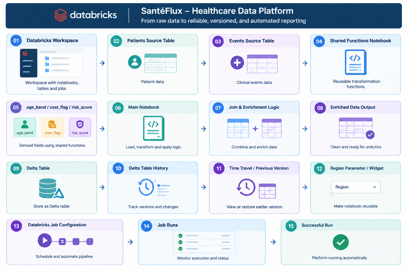
SanteFlux Healthcare Data Platform diagram, 15 numbered steps: Databricks workspace, Patients source table, Events source table, Shared Functions Notebook, age_band, cost_flag and risk_score, Main Notebook, Join and Enrichment Logic, Enriched Data Output, Delta Table, Delta Table History, Time Travel and Previous Version, Region Parameter and Widget, Databricks Job Configuration, Job Runs, and Successful Run. — The whole build in one diagram: two source tables, a shared-functions notebook, a main notebook that joins and enriches, a Delta table with history, and the job that schedules it.

Set up the catalog, then read the data

Everything lives under one catalog, with its own schema and volume, so the platform has a governed home before a single row is read.

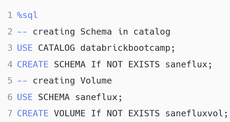
SQL cell: USE CATALOG databrickbootcamp, CREATE SCHEMA IF NOT EXISTS saneflux, USE SCHEMA saneflux, CREATE VOLUME IF NOT EXISTS sanefluxvol. — One schema, one volume, created once and reused by every notebook that follows.

PySpark notebook cell importing libraries: from pyspark.sql.functions import star. — The only import the functions notebook needs.

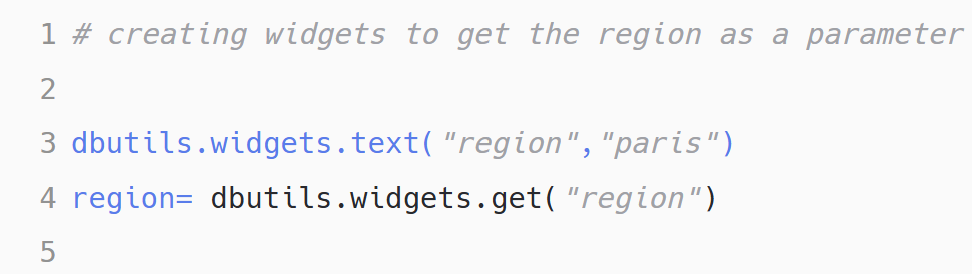
Notebook cell creating a widget: dbutils.widgets.text(region, paris), then region equals dbutils.widgets.get(region). — The region parameter, created as a widget from the first cell, defaulting to Paris but overridable by whatever calls the notebook.

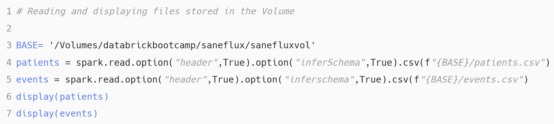
Notebook cell setting BASE to a Volumes path, then reading patients and events as CSVs with header and inferSchema options, and displaying both. — Both source files read from the governed volume, with Spark inferring their schema rather than treating every column as text.

Patients table sample: patient_id, full_name, date_of_birth, home_address, diagnosis_code, region, gp_email columns, rows including Zoe Guerin in Nice with diagnosis J45 and Emma Mercier in Nice with diagnosis E11.9. — One row per person, including the identifying fields the platform will carry through every layer untouched: name, address, GP email.

Events table sample: event_id, patient_id, event_date, event_ts, event_type, department, region columns, rows spanning laboratoire, prescription and consultation event types across Rouen, Lyon, Paris. — One row per clinical episode, each carrying its own region, the field the join has to handle carefully.

Shared functions: write the rule once

Three fields, each a plain function that takes a column and returns a column, so the logic exists in exactly one place rather than copied into whichever notebook needs it.

PySpark function age_band(dob_col): computes age from datediff against current_date divided by 365.25, then returns a chained when expression banding it into 0-17, 18-39, 40-64, or 65+. — age_band, banded from date of birth exactly as the brief specified.

PySpark function cost_flag(amount_col): returns when amount_col is greater than or equal to 50, high, otherwise normal. — cost_flag, a single threshold turned into a named, reusable rule.

PySpark function risk_score(dob_col, diag_col, amount_col): sums 2 points when age_band returns 65+, 2 points when cost_flag returns high, and 2 points when the diagnosis code starts with E11.9 or I10, otherwise 0 for each. — risk_score calls age_band and cost_flag directly rather than re-deriving them, which is the entire argument for naming the first two functions in the first place.

Challenge 01

Keep the join from producing two columns with one name

Both patients and events carry a region column, patients recording where someone lives, events recording where the episode happened. A plain join on patient_id leaves both in the result, ambiguous to any downstream query that references region, and the two values won't always agree for a patient treated outside their home area.

The join keeps events.region and explicitly drops patients.region before the two tables ever collide:

joined_df = patients.join(events,"patient_id","left").drop(patients.region)

That’s a business decision as much as a syntax fix. SantéFlux’s board wants regional cost and trend figures, and the region that determines which provider incurred the cost is where the episode happened, not necessarily where the patient’s address is registered. Dropping the patient’s copy keeps the surviving region column unambiguous for every function and every report built on top of joined_df, and it keeps that column meaning the same thing every time someone reads it.

Notebook cell running the magic command percent-run, pointing at the SanteFlux_Functions notebook inside the author's Databricks workspace, with a comment explaining that percent-run executes a helper notebook in the background so its functions become available. — The main notebook pulls in every function from the shared notebook with one %run line, rather than copying the three definitions across.

PySpark cell: joined_df equals patients.join(events, patient_id, left).drop(patients.region), with a comment noting the drop resolves column ambiguity, followed by display(joined_df). — One join, one drop, and the region collision is resolved before anything downstream ever sees it.

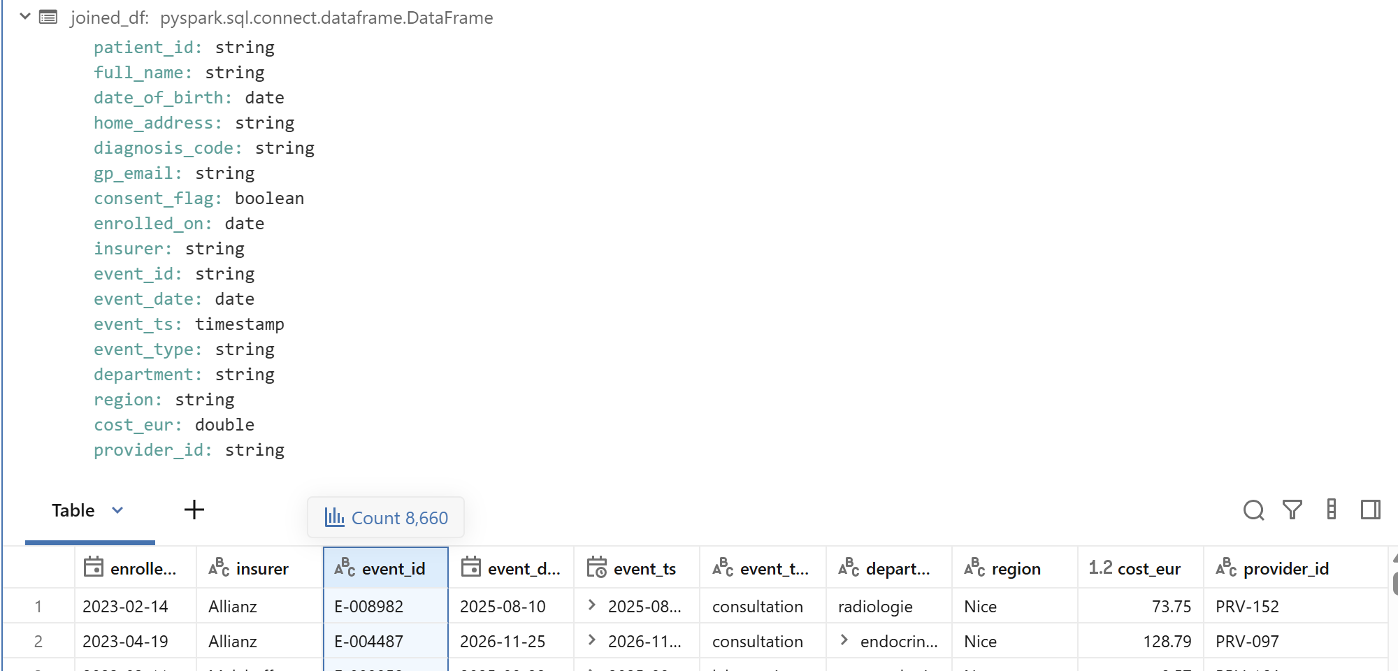
joined_df schema listing patient_id, full_name, date_of_birth, home_address, diagnosis_code, gp_email, consent_flag, enrolled_on, insurer, event_id, event_date, event_ts, event_type, department, region, cost_eur and provider_id, region appearing exactly once, and a data grid below it with a row count of 8,660. — Region appears exactly once in the schema, and the join produced 8,660 enriched episodes, proof the drop worked rather than an assumption.

Enrich, then look at it three different ways

The three shared functions get applied to the joined data in one chained expression, then the result gets inspected with print, show and display, a deliberate comparison of what each actually returns.

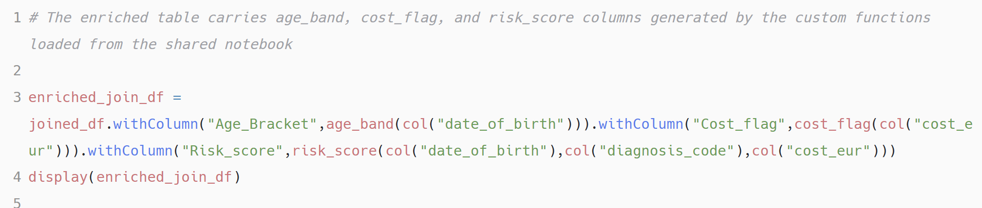
PySpark cell: enriched_join_df equals joined_df.withColumn(Age_Bracket, age_band(col(date_of_birth))).withColumn(Cost_flag, cost_flag(col(cost_eur))).withColumn(Risk_score, risk_score(col(date_of_birth), col(diagnosis_code), col(cost_eur))), then display(enriched_join_df). — Three withColumn calls, each invoking a shared function rather than inlining the rule again.

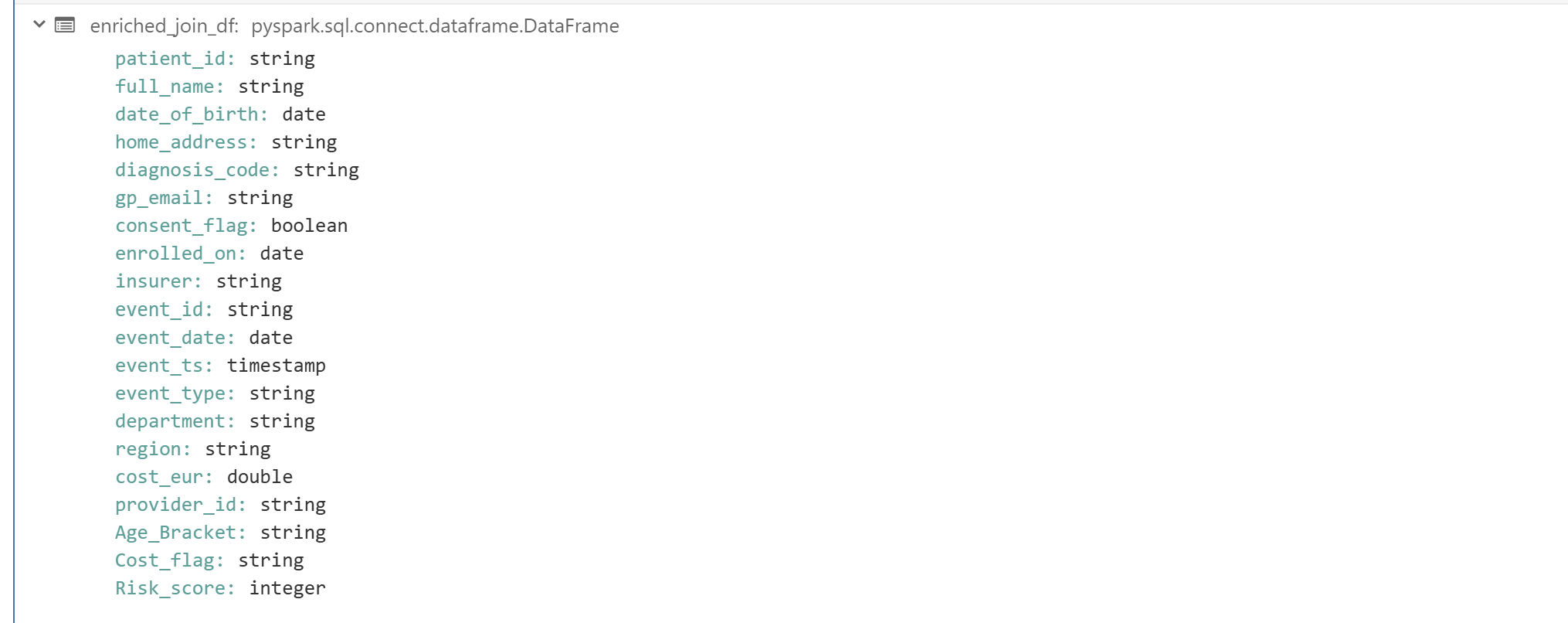
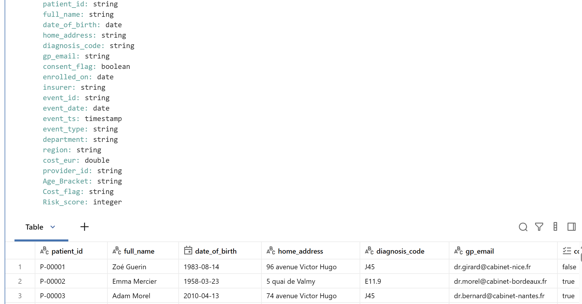
enriched_join_df schema listing every column from the join plus Age_Bracket as string, Cost_flag as string, and Risk_score as integer. — Three new columns added, nothing else disturbed.

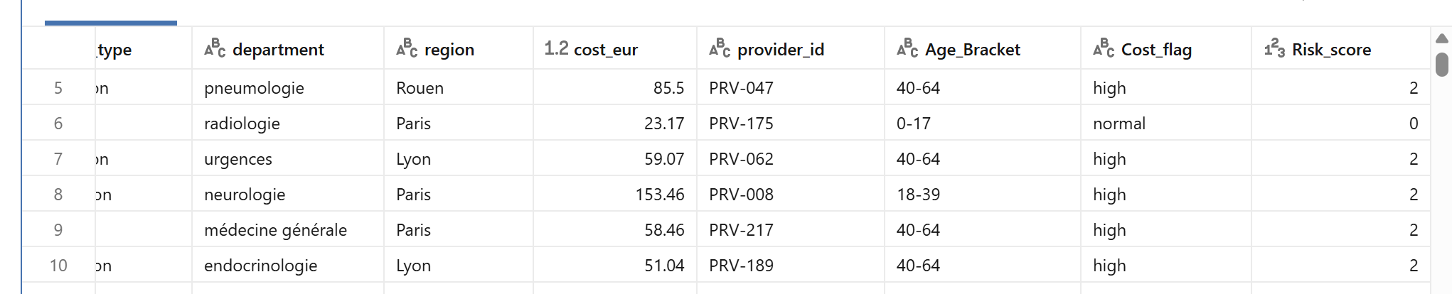
Enriched result sample: department, region, cost_eur, provider_id, Age_Bracket, Cost_flag, Risk_score columns, rows showing a 40-64 year-old with cost_eur 85.5 flagged high and a risk score of 2, alongside a 0-17 year-old with cost_eur 23.17 flagged normal and a risk score of 0. — risk_score doing exactly what the derivation contract specified: the 65+ or high-cost row scores 2, the young, low-cost row scores 0.

print(enriched_join_df) output: DataFrame[patient_id: string, full_name: string, date_of_birth: date, home_address: string, diagnosis_code: string, region: string, gp_email: string, ...] listing every column and its type as plain text. — print() shows the schema, nothing more, a plan rather than data.

enriched_join_df.show() output: a monospaced text table with pipe-separated columns for patient_id, full_name, date_of_birth, home_address, diagnosis_code, region, gp_email and more, rows for Zoe Guerin, Emma Mercier and Adam Morel. — show() renders an actual text-based preview of the rows, truncated to fit the console width.

display(enriched_join_df.limit(5)) output: an interactive graphical table with patient_id, full_name, date_of_birth, home_address, diagnosis_code, region and gp_email columns, showing Zoe Guerin at 96 avenue Victor Hugo and Emma Mercier at 5 quai de Valmy, both in Nice. — display() is the one built for exploration: sortable, filterable, and the version every screenshot in this write-up after this point uses.

A quick regional count, three ways to have written it

Before writing the table, the notebook checks how many events landed in each region, a small aside that’s really about knowing when it’s safe to pull data back to the driver.

PySpark cell: region_rows equals enriched_join_df.select(region).distinct().collect(), then print(region_rows) and print(region_rows[0][0]). — Eight distinct regions, collected to the driver. Safe here because distinct() has already reduced millions of rows down to eight before collect() ever runs.

Output: a list of eight Row objects, region equal to Rouen, Toulouse, Nantes, Paris, Marseille, Bordeaux, Nice and Lyon, followed by Rouen printed twice, once as a plain string and once quoted. — All eight regions, exactly as many as SantéFlux operates in.

PySpark cell: region_values equals an empty list, then a for loop over region_rows appending y［0］ to region_values, then printing it. — Unwrapping each Row into a plain string, ready to drive a Python loop.

Output: a plain Python list, Rouen, Toulouse, Nantes, Paris, Marseille, Bordeaux, Nice, Lyon. — Eight strings, no longer wrapped in Spark Row objects.

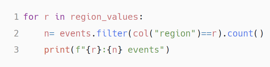
PySpark cell: a for loop over region_values, filtering events to that region and counting, then printing the region and its event count. — One filter and count per region, run from the Python side rather than as a single grouped aggregation, a fair trade at eight regions, one that stops paying off once the region list is one you can't type into a loop.

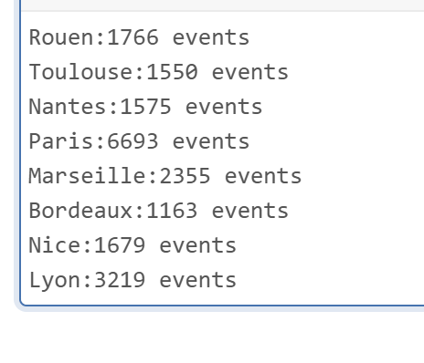
Output: Rouen 1766 events, Toulouse 1550 events, Nantes 1575 events, Paris 6693 events, Marseille 2355 events, Bordeaux 1163 events, Nice 1679 events, Lyon 3219 events. — Paris alone accounts for a third of all events, and the eight totals add up to exactly 20,000, the full extract accounted for.

Version the table, prove the rollback

The enriched result is written as a managed Delta table, and every subsequent write becomes a version rather than a replacement.

PySpark cell: enriched_join_df.write.mode(overwrite).saveAsTable(databrickbootcamp.saneflux.patient_risk), with a comment reading writing enriched df as delta. — The first write, creating databrickbootcamp.saneflux.patient_risk as a managed Delta table.

PySpark cell reading the table back: df equals spark.read.table(databrickbootcamp.saneflux.patient_risk), then display(df). — Reading the table back to confirm it landed.

patient_risk table schema and sample rows: patient_id, full_name, date_of_birth, home_address, diagnosis_code, gp_email, consent_flag and every enriched column, rows for Zoe Guerin, Emma Mercier and Adam Morel with their consent_flag values. — The versioned table, holding the same patient-identifying columns the source files carried in, untouched by anything in this build.

To prove the rollback actually works, the next cell deliberately breaks the table: every risk score in the entire dataset gets set to zero, no WHERE clause, the exact kind of Thursday-morning mistake the brief opened with.

SQL cell: UPDATE databrickbootcamp.saneflux.patient_risk SET Risk_score = 0, with a comment reading update the risk scores to zero across the entire patient risk dataset. — A deliberate, unqualified UPDATE, the bad change the rest of this section exists to recover from.

SQL cell: DESCRIBE HISTORY databrickbootcamp.saneflux.patient_risk, with a comment reading check the transaction and version history of the delta table. — Asking Delta for the table's full write history.

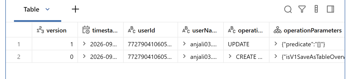
History result: two rows, version 1 with operation UPDATE and operationParameters predicate empty brackets (confirming no WHERE clause), version 0 with operation CREATE, both attributed to the same userId and userName. — Version 1 is the damage, right there in the operationParameters: an empty predicate means every row matched. Version 0 is what the RESTORE below reaches back for.

SQL cell: RESTORE TABLE databrickbootcamp.saneflux.patient_risk TO VERSION AS OF 0, with a comment reading restore the delta table back to its initial version 0 to undo the risk score updates. — One statement, no backup file, no re-running the pipeline: the table returns to exactly what it held before the bad update, and the RESTORE itself becomes version 2 rather than erasing version 1 from the record.

Schedule the job

The last step turns the region widget into a job parameter and wires the main notebook to a Databricks Job on a daily trigger, so the platform runs whether or not an engineer is watching.

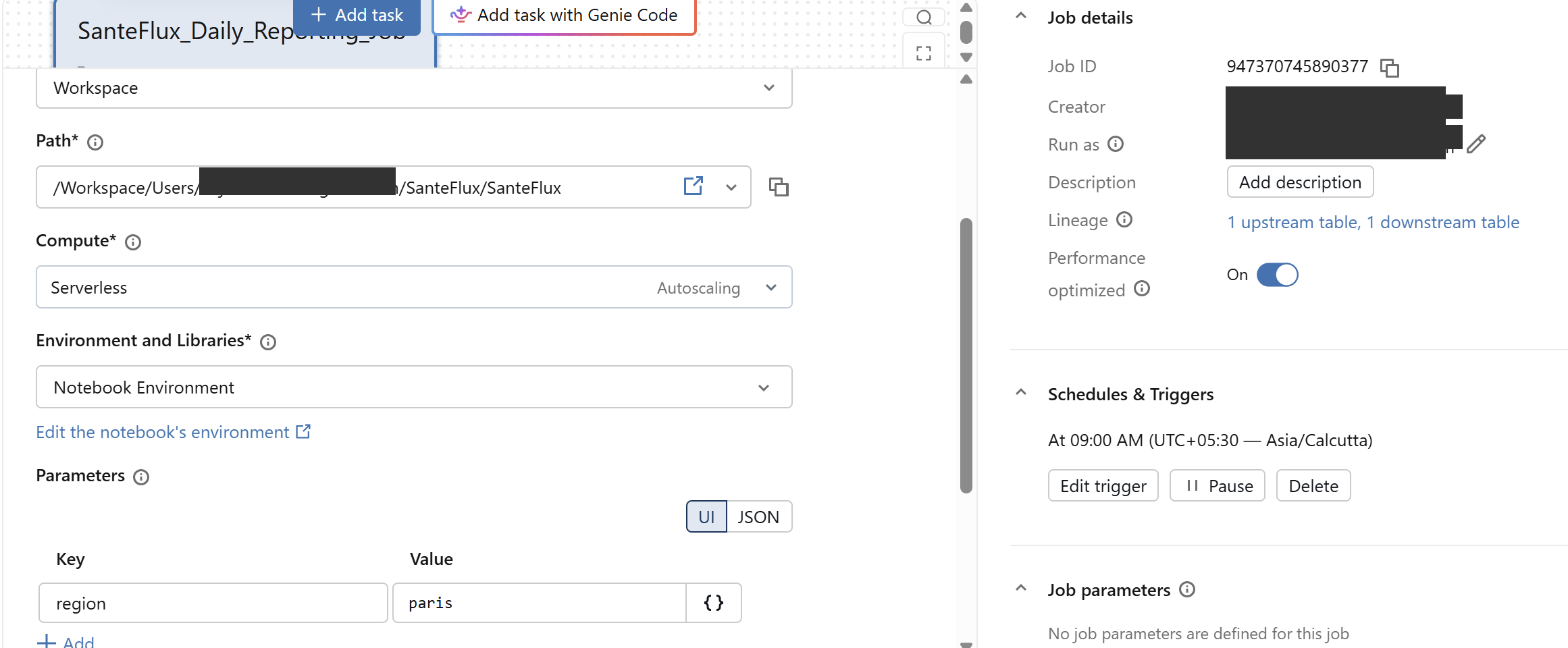
Databricks Job configuration for SanteFlux_Daily_Reporting_Job: Compute Serverless, Parameters key region value paris, Job details showing Job ID, Lineage of 1 upstream and 1 downstream table, Schedules and Triggers set to 09:00 AM UTC+05:30 Asia/Calcutta, and Job parameters. — The region parameter set at the job level rather than typed into a cell, and a daily 09:00 trigger, both proof the run no longer depends on a person.

The schedule itself is worth a second look: it’s set to 09:00 in the workspace’s own timezone, Asia/Calcutta, rather than Europe/Paris. Harmless for a bootcamp job, but exactly the kind of detail that needs fixing before this platform actually reports on the morning a Paris care provider is expecting, not the morning IST happens to deliver it.

What this proves

Reuse, then history, then automation, in that order, because reversing it ships the fragility it was meant to remove: functions shared before the join means a corrected rule lands everywhere at once, the table versioned before it’s trusted means a Thursday mistake is a RESTORE away from Wednesday, and the run handed to a schedule last means neither of the first two matter if someone still has to remember to press the cells.