Workforce Intelligence: Azure SQL to Lakehouse
Retiring a manual SQL export and an Excel cleaning ritual that cost HR two days of reporting latency.
This project implements a modern Microsoft Fabric data engineering pipeline that transforms raw workforce data into a trusted analytical dataset for Human Resources reporting.
The solution replaces a manual SQL export and Excel-based reporting workflow with an automated Bronze-to-Silver Lakehouse architecture built using Microsoft Fabric, Azure SQL Database, and PySpark. The pipeline emphasises data quality, auditability, incremental processing, and reusable transformation logic.
The business problem
The HR department relied on:
- Manual SQL exports
- Excel-based cleaning
- Duplicate employee records
- Invalid salary values
- Missing hire dates
- No governed analytical layer
- Approximately 48-hour reporting delays
The objective was to design a scalable Microsoft Fabric solution capable of producing clean, trusted workforce data for downstream reporting.
Solution architecture
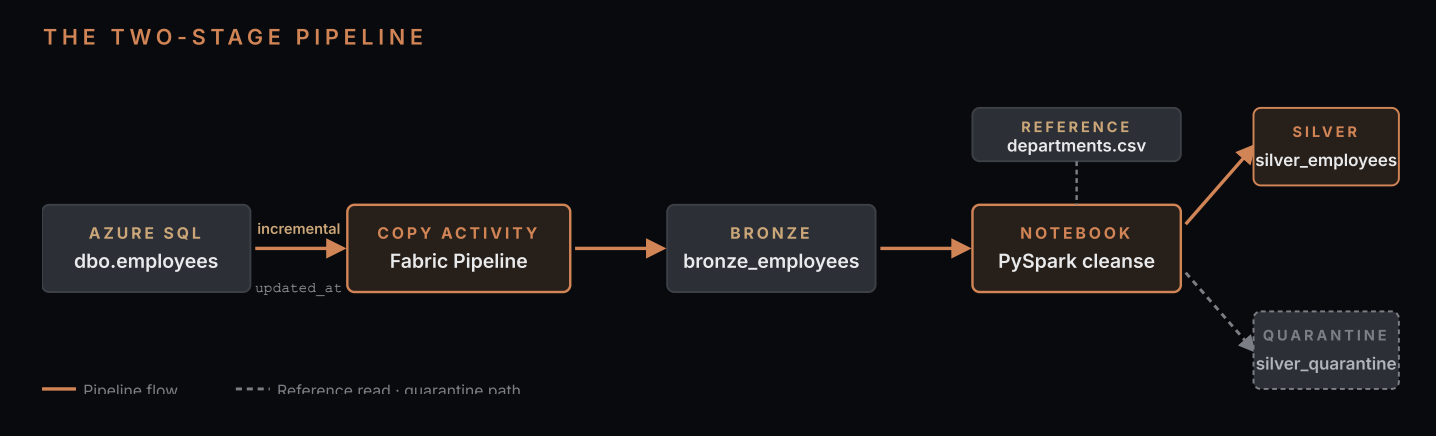 View full size (opens in a new tab)
Data quality challenges
The source system contained multiple quality issues that required cleansing before analytics.
| Issue | Resolution |
|---|---|
| Null hire dates | Quarantined |
| Null salaries | Quarantined |
| Invalid salary values | Quarantined |
| Duplicate employee IDs | Retained latest record using updated_at |
| Name prefixes | Extracted into a separate column |
| Missing analytics layer | Bronze–Silver architecture |
Quarantining rather than deleting is the decision that matters here. A dropped row is a number nobody can reconcile later; a quarantined row is a number someone can go and fix.
Extra challenges
- Bonus 01: Rank
- Bonus 02: Compare
- Bonus 03: Aggregate
Solution
Step 1: Inspect
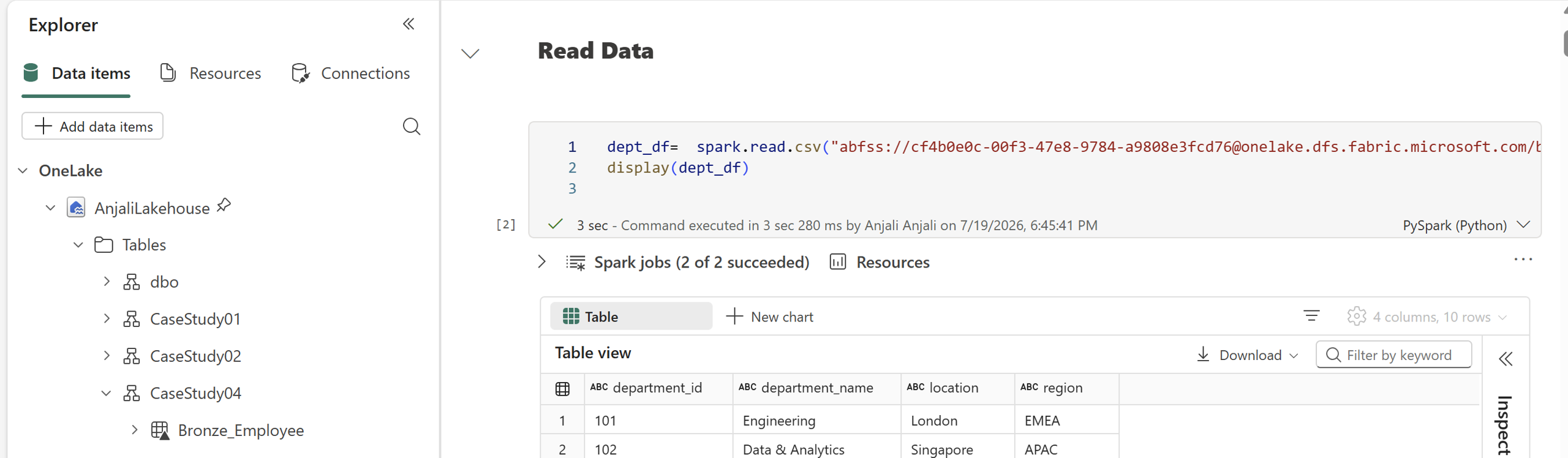
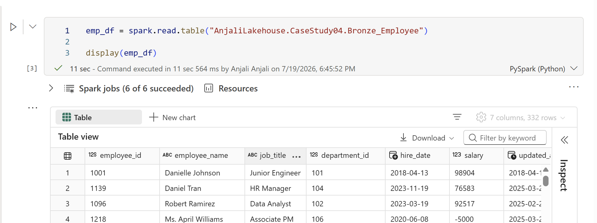
Profile the raw Bronze table and the department reference data, and establish row counts before any change.
- spark.read.csv()
- Loads raw CSV data into a PySpark DataFrame by parsing structural parameters like delimiters and headers.
- display()
- A native Fabric utility that renders DataFrames into interactive visual tables for quick profiling.
- spark.read.table()
- Loads data directly from a registered Lakehouse Delta table into a PySpark DataFrame.
 View full size (opens in a new tab)
 View full size (opens in a new tab)
Step 2: Quarantine
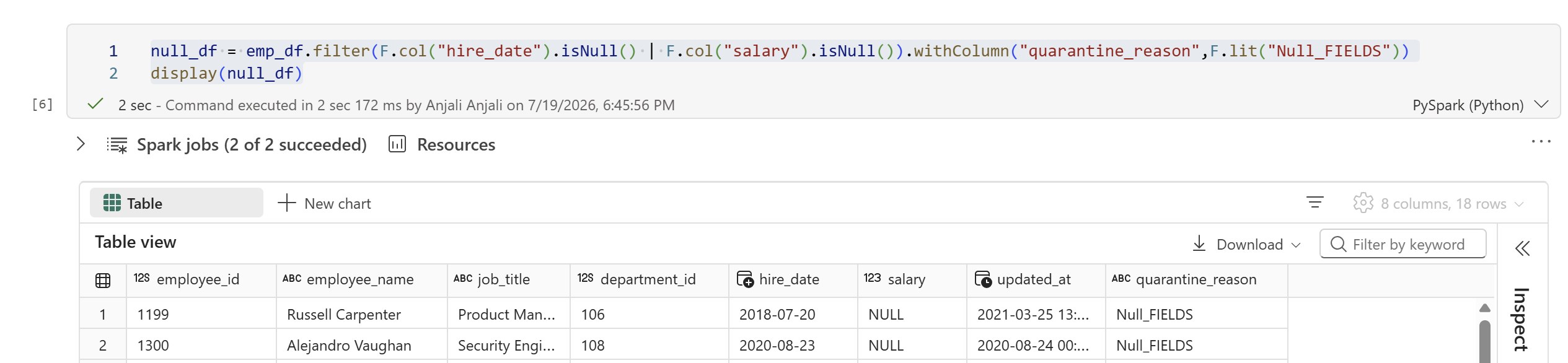
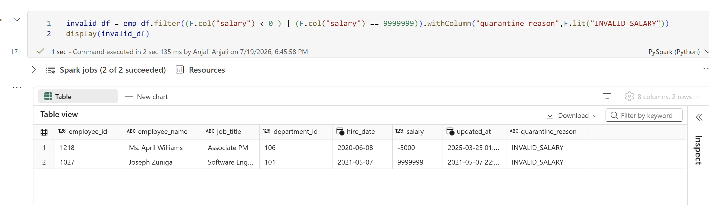
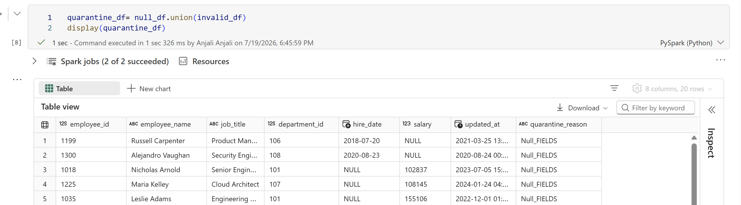
Filter out null hire dates, null salaries, and invalid salary values, tagging each with its rejection reason and unioning them into a quarantine table.
- from pyspark.sql import functions as F
- Imports the PySpark SQL functions library, providing access to the transformation, aggregation, and manipulation methods used throughout the pipeline.
- .filter()
- Filters rows in a DataFrame based on specified conditions, retaining only the records that meet the criteria.
- F.col()
- References a specific column in the DataFrame by its name to apply expressions or transformations.
- .isNull()
- Evaluates column values and returns true if a record contains a missing or null value.
- | (bitwise OR)
- Combines multiple filter conditions, returning rows where at least one of the conditions evaluates to true.
- .withColumn()
- Creates a new column or replaces an existing one by applying a transformation or assigning a value.
- F.lit()
- Creates a literal or constant value column, allowing static text or numbers to be appended to every row.
- .union()
- Combines two DataFrames vertically by appending the rows of one to another, requiring both to share the same schema structure.
- .write
- Accesses the DataFrameWriter interface used to save DataFrame contents to external storage or a metastore.
- .mode("Overwrite")
- Specifies the save behaviour, configured to completely replace any existing data and schema in the target destination.
- .saveAsTable()
- Persists the DataFrame directly into the Lakehouse metastore as a managed Delta table at the specified path.
 View full size (opens in a new tab)
 View full size (opens in a new tab)
 View full size (opens in a new tab)
 View full size (opens in a new tab)
Step 3: Deduplicate
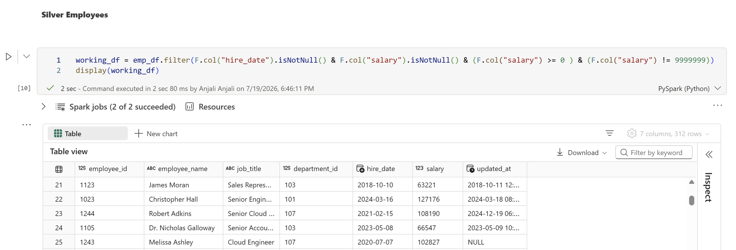
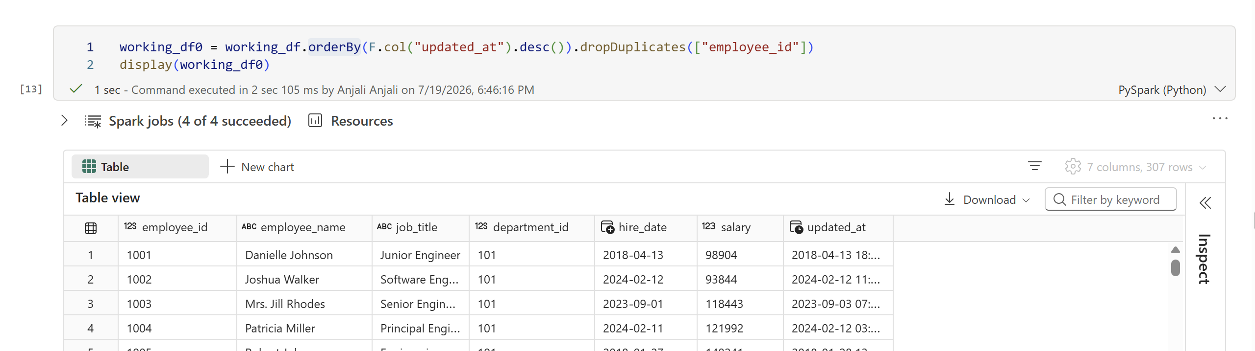
Keep only valid records, then order by updated_at descending and drop duplicates on
employee_id, keeping the most recent record for each employee.
- .isNotNull()
- Evaluates column values, keeping only those that contain valid, non-null data.
- & (bitwise AND)
- Combines multiple filter conditions, ensuring only rows meeting all specified criteria remain.
- .orderBy(..., .desc())
- Sorts the DataFrame by a specific column in descending order, ensuring the most recent entries appear first.
- .dropDuplicates()
- Identifies and removes duplicate records based on the specified column, in this case
employee_id, retaining only the first and therefore latest occurrence.
 View full size (opens in a new tab)
 View full size (opens in a new tab)
Steps 4 to 6: Enrich, join, stamp and write
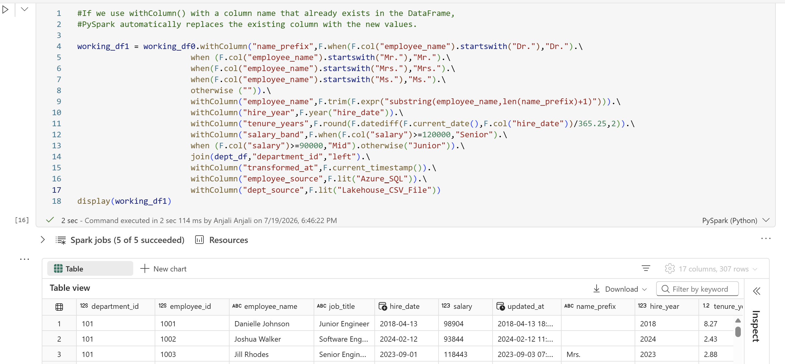
Extract name prefixes, derive hire year, tenure and salary band, join the department reference data, stamp audit columns, and write the governed Silver table. The bulk of the work happens in a single chained expression:
working_df1 = working_df0.withColumn("name_prefix", F.when(F.col("employee_name").startswith("Dr."), "Dr.")
                    .when(F.col("employee_name").startswith("Mr."), "Mr.")
                    .when(F.col("employee_name").startswith("Mrs."), "Mrs.")
                    .when(F.col("employee_name").startswith("Ms."), "Ms.")
                    .otherwise("")) \
    .withColumn("employee_name", F.trim(F.expr("substring(employee_name, len(name_prefix)+1)"))) \
    .withColumn("hire_year", F.year("hire_date")) \
    .withColumn("tenure_years", F.round(F.datediff(F.current_date(), F.col("hire_date")) / 365.25, 2)) \
    .withColumn("salary_band", F.when(F.col("salary") >= 120000, "Senior")
                    .when(F.col("salary") >= 90000, "Mid").otherwise("Junior")) \
    .join(dept_df, "department_id", "left") \
    .withColumn("transformed_at", F.current_timestamp()) \
    .withColumn("employee_source", F.lit("Azure_SQL")) \
    .withColumn("dept_source", F.lit("Lakehouse_CSV_File"))
The employee_source and dept_source literals are deliberate: six months later, when a
number looks wrong, the Silver table itself says which system it came from.
- .withColumn()
- Adds or replaces a column by applying a transformation expression; overwrites an existing column if the same name is provided.
- F.when().otherwise()
- Implements conditional logic similar to an IF-ELSE statement to assign values based on specific criteria.
- F.trim()
- Removes leading and trailing whitespace from a string column.
- F.expr("substring(...)")
- Executes a SQL-style substring expression to extract portions of text data.
- F.round()
- Rounds a numeric value to a specified number of decimal places.
- F.year()
- Extracts the year component from a date or timestamp column.
- F.datediff()
- Calculates the difference in days between two date or timestamp columns.
- F.current_date()
- Returns the current system date as a date type.
- F.current_timestamp()
- Returns the current system timestamp.
- F.lit()
- Creates a column with a constant, static literal value for every row.
- .join(..., "left")
- Combines two DataFrames on a shared key column using a left-outer join, keeping all records from the left DataFrame.
 View full size (opens in a new tab)
 View full size (opens in a new tab)
Step 7: Reconcile
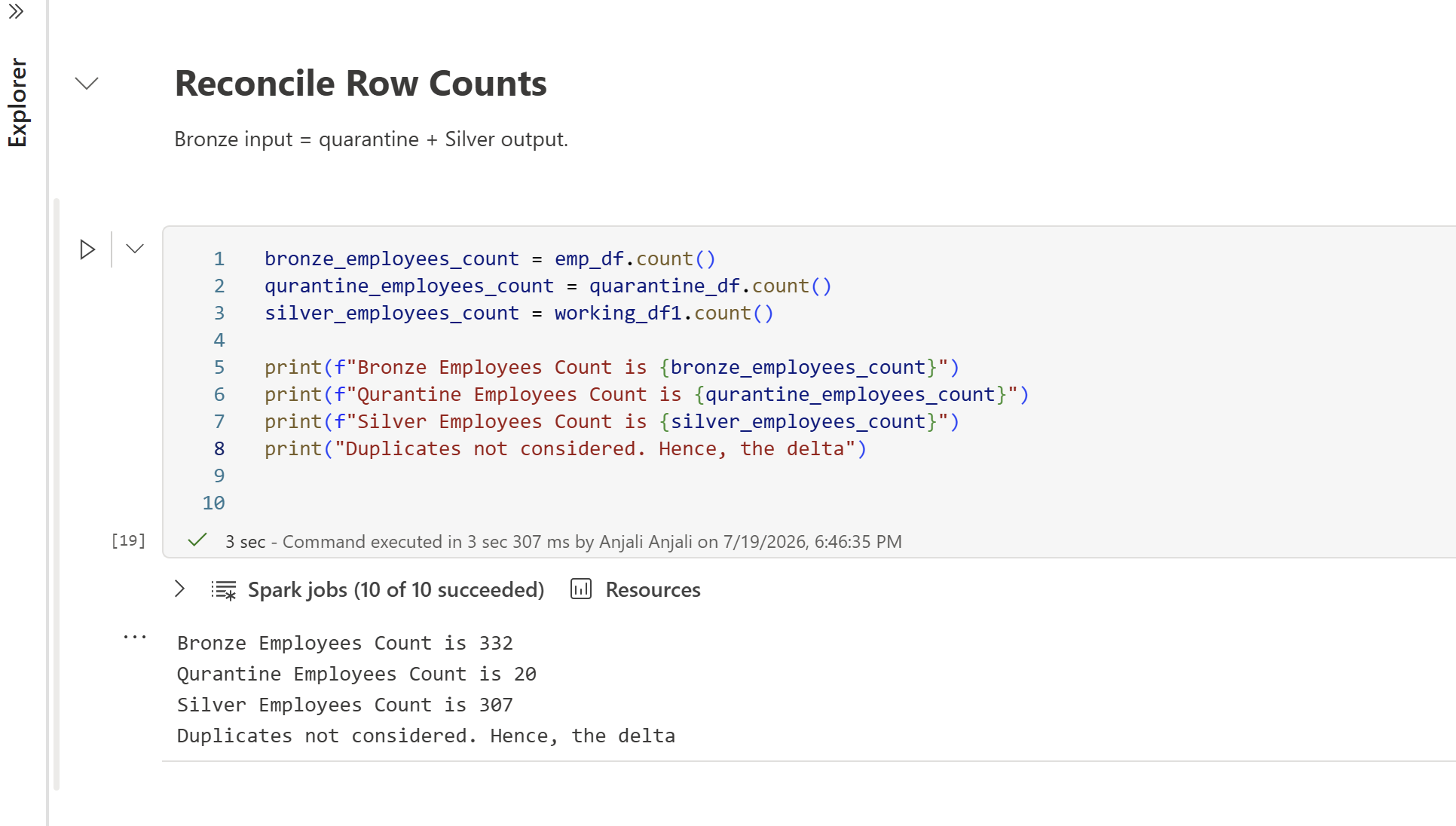
Count rows across every stage so Bronze, Silver, and quarantine always add up.
 View full size (opens in a new tab)
- .count()
- A PySpark action that calculates and returns the total number of rows in a DataFrame, essential for auditing data volumes across pipeline stages.
- print(f"...")
- A standard Python function using f-strings to format and display text alongside calculated variable values for quick output logging.
Bonus challenge solutions
Three HR questions that each need a window function rather than a group-by.
Bonus 01: Salary rank within department
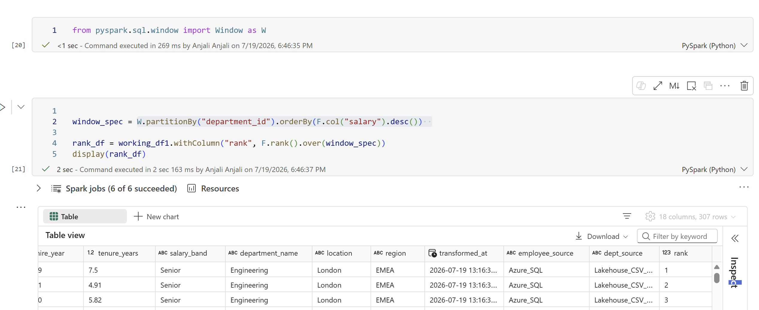
HR wants to know where each employee ranks within their department by salary. Produce a ranking that resets for each department. Handle tied salaries fairly: the same salary should produce the same rank.
 View full size (opens in a new tab)
- W.partitionBy()
- Defines the window boundary by grouping the data into logical partitions, for example by
department_id, so that window functions likerank()are calculated independently within each group. - .orderBy(F.col("column_name").desc())
- Specifies the sorting order within each window partition, arranging records by the target column from highest to lowest.
- F.rank().over(window_spec)
- Assigns a rank to each row within the defined partition, where tied values receive the same rank and the sequence skips numbers accordingly, for example 1, 2, 2, 4.
Bonus 02: Salary versus department average
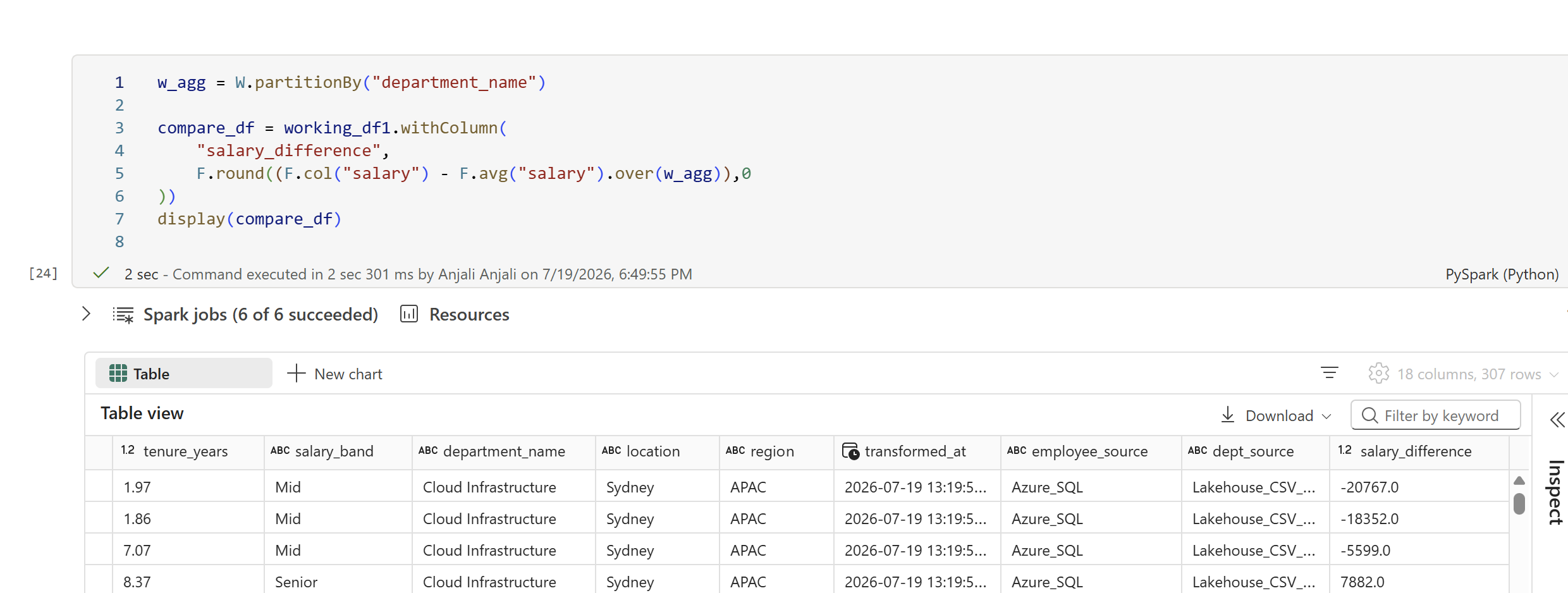
HR wants to understand how each employee’s salary compares to the average in their department. Add a new column showing the difference. A positive value means above average. A negative value means below.
 View full size (opens in a new tab)
- W.partitionBy()
- Defines the window boundary by grouping the data into logical partitions, for example by
department_name, so that window functions likeavg()are calculated independently within each group. - F.round((F.col("salary") - F.avg("salary").over(w_agg)), 0)
- Calculates the variance between an individual’s salary and their department’s average salary, rounding the resulting difference to the nearest whole number.
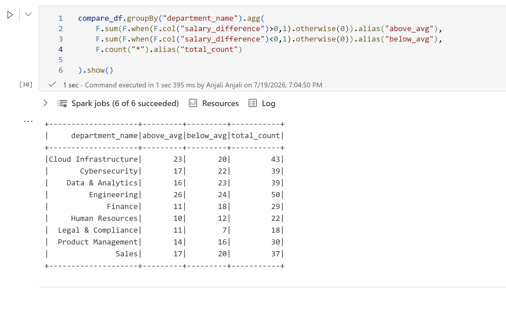
To validate the analytical results, the data is grouped by department to calculate the frequency of salaries above and below the department average, alongside total headcounts per department. If those counts do not sum to the headcount, the window is wrong.
 View full size (opens in a new tab)
- .groupBy("column_name")
- Clusters rows by department to enable aggregate calculations for each group.
- F.sum(…)
- Aggregates conditional counts to total how many employees fall above or below the department average.
- F.count("*")
- Calculates the total number of records within each department grouping.
- .alias(…)
- Renames resulting aggregate columns to provide clear, readable labels in the final table.
Bonus 03: Top earner per region
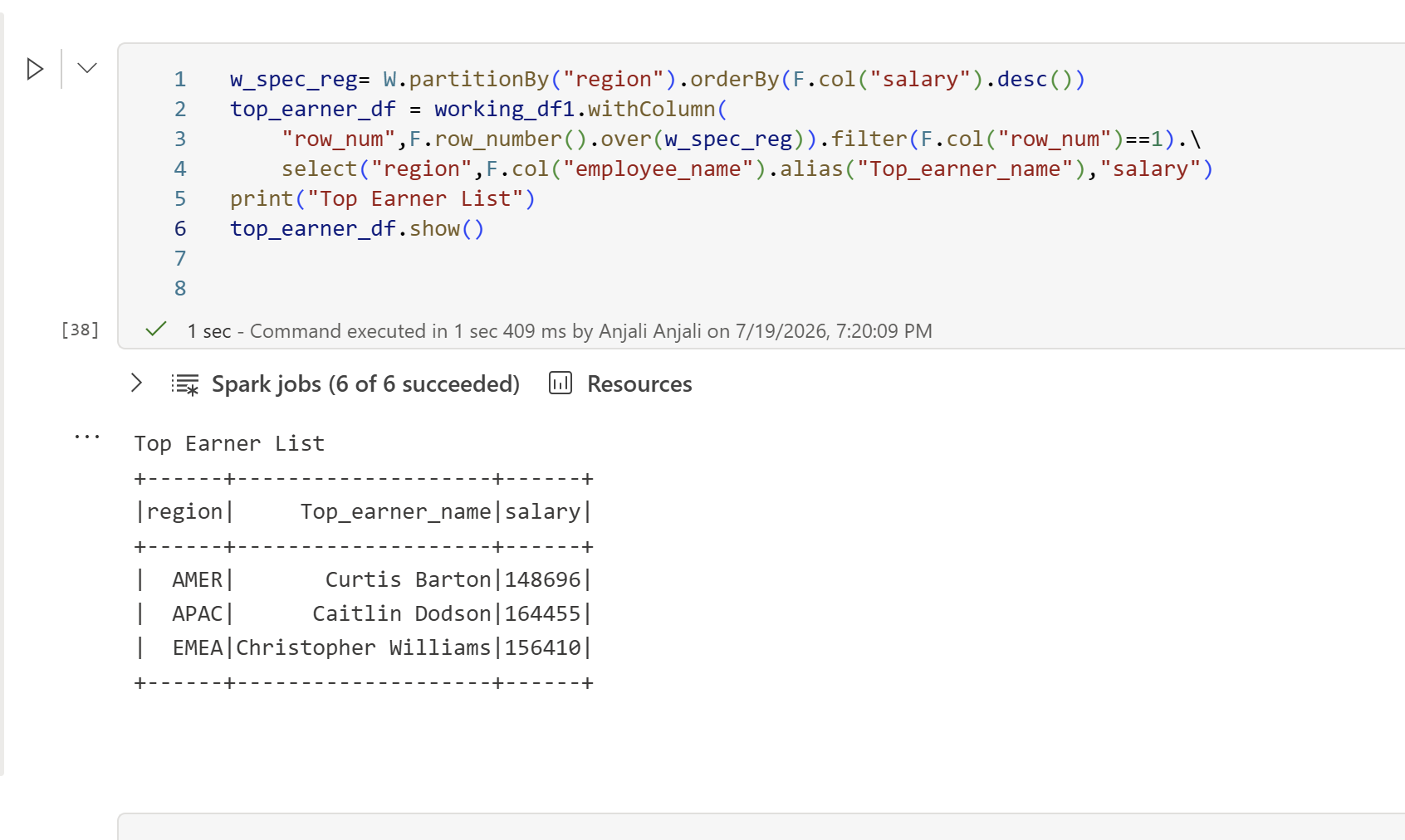
The HR Director wants to know who earns the most in each region. Your solution must work regardless of how many regions exist in the data. Do not hardcode the region count.
 View full size (opens in a new tab)
- W.partitionBy("region").orderBy(...)
- Groups the data by region and sorts salaries in descending order within each group to identify the highest earner.
- F.row_number().over(w_spec_reg)
- Assigns a unique, sequential number to each row within the region, ensuring the top earner always receives a 1.
- .filter(F.col("row_num") == 1)
- Selects only the records where the row number is 1, isolating the top earner for every region.
- .select("region", F.col("...").alias("..."), "salary")
- Retains only the necessary columns while renaming the employee name column for clear, professional reporting.