Financial Data Transformation
Making engineering decisions from execution-plan evidence rather than intuition.
Designed and optimised a financial data processing pipeline in Microsoft Fabric using PySpark and Delta Lake. The project focused on improving pipeline performance, enforcing data quality, enabling data recovery, and building a scalable architecture for enterprise-scale financial reporting.
The business problem
A multinational finance division relied on a daily Accounts Receivable (AR) reporting pipeline that processed 45 million transaction records by joining them with a 15,000-record customer master table.
The existing pipeline faced several challenges:
- Processing time exceeded 2 hours
- Large data shuffling caused poor Spark performance
- Invalid data was loaded because schema validation was missing
- Corrupted data reached executive dashboards
- No mechanism existed to recover previous versions after bad data loads
- Growing data volumes reduced query performance
- Manual recovery increased operational risk and compliance concerns
Key objectives
The project aimed to:
- Reduce pipeline execution time
- Optimise PySpark joins for large datasets
- Improve data quality through schema validation
- Enable version control and data recovery
- Build a scalable and maintainable data pipeline
- Improve query performance for analytical reporting
- Support governance, auditing, and compliance requirements
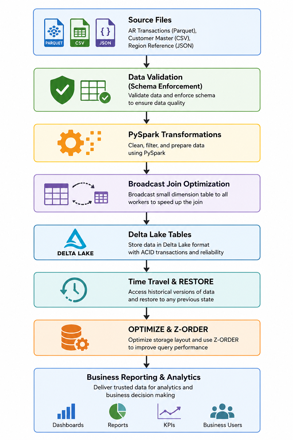
Solution architecture
 View full size (opens in a new tab)
- Source files: raw financial data is collected from multiple sources, including transaction records, customer master data, and reference datasets, to support downstream processing.
- Data validation (schema enforcement): incoming data is validated against predefined schemas to ensure only accurate and properly formatted records enter the pipeline.
- PySpark transformations: data is cleaned, transformed, and prepared using PySpark to create a structured dataset for analysis and reporting.
- Broadcast join optimisation: the customer master table is broadcast to all worker nodes, reducing data shuffling and significantly improving join performance.
- Delta Lake tables: processed data is stored in Delta Lake tables, providing ACID transactions, schema enforcement, and reliable version control.
- Time Travel and RESTORE: Delta Lake’s version history is used to view previous table states and quickly restore data if an incorrect or failed load occurs.
- OPTIMIZE and Z-ORDER: data files are compacted and reorganised to improve storage efficiency and speed up queries on large datasets.
- Business reporting and analytics: the optimised and trusted data is delivered to business users for accurate reporting, dashboard creation, and data-driven decision-making.
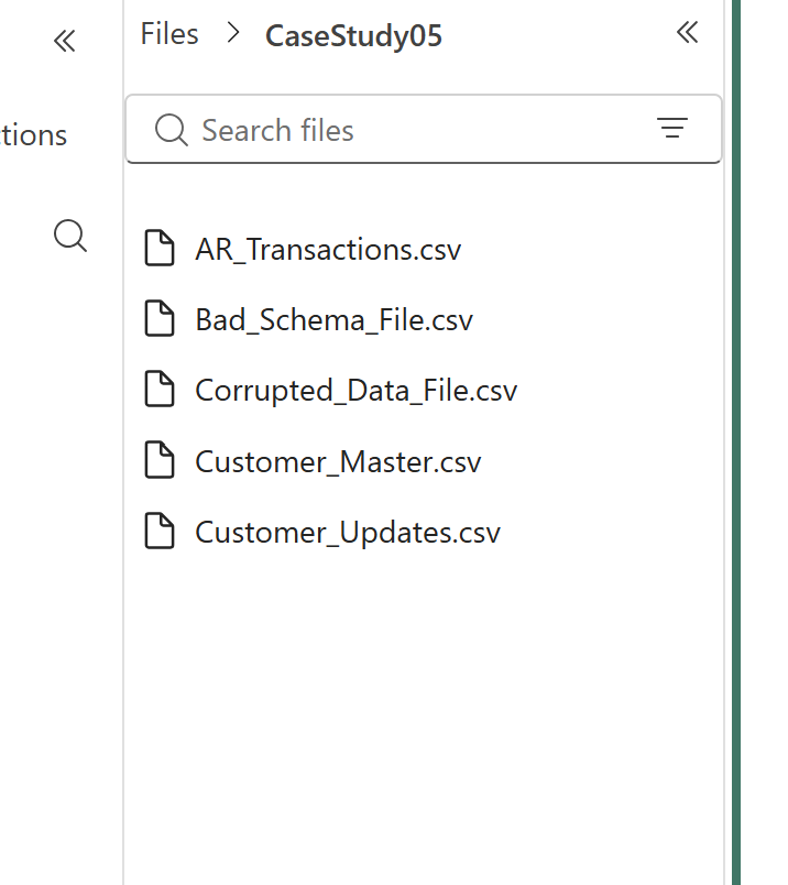
Step 1: Define the schema and load the data
 View full size (opens in a new tab)
Rather than letting Spark infer types, the structure of each dataset is stated explicitly:
transaction_schema = StructType([
StructField("TransactionID", StringType(), False),
StructField("CustomerID", StringType(), True),
StructField("Transaction_Date", DateType(), True),
StructField("TransactionAmount", FloatType(), True),
])
Customer_schema = StructType([
StructField("CustomerID", StringType(), False),
StructField("CustomerNames", StringType(), True),
StructField("Address", StringType(), True),
StructField("Credit_Limit", FloatType(), True),
])
transaction_df = spark.read.csv('Files/CaseStudy05/AR_Transactions.csv', header=True, schema=transaction_schema)
customer_master_df = spark.read.csv('Files/CaseStudy05/Customer_Master.csv', header=True, schema=Customer_schema)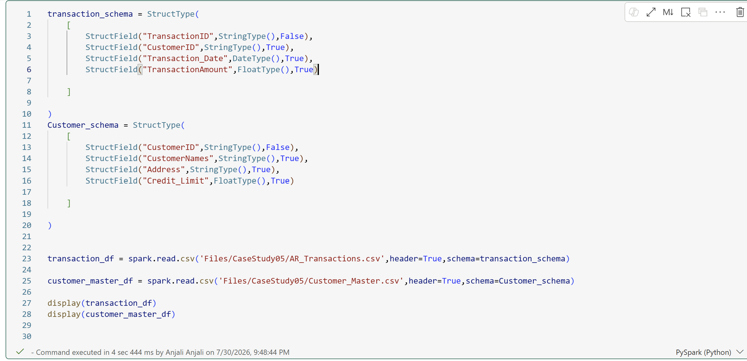 View full size (opens in a new tab)
What are we doing? Defining the schema for the AR Transactions and Customer Master datasets before loading them into PySpark DataFrames. Instead of allowing Spark to detect the data types automatically, the structure of each dataset is specified explicitly to ensure consistent and accurate data ingestion.
Why are we doing this? Defining the schema improves data quality by preventing incorrect data types, avoids errors caused by automatic schema inference, and speeds up loading, because Spark no longer needs to examine the entire dataset to determine column types. On 45 million rows, that scan is not free. This creates a reliable foundation for all downstream transformations and analysis.
Functions used
- StructType()
- Creates the overall schema for a DataFrame by grouping all column definitions together.
- StructField()
- Defines the properties of an individual column, including its name, data type, and whether it can contain null values.
- schema=
- Applies the predefined schema while reading the file, ensuring the correct data types are assigned to each column.
- inferSchema=True
- The alternative: Spark examines the data and determines the appropriate type for each column, such as Integer, String, Date or Float, removing the need to define the schema manually but costing an extra pass over the dataset.
Step 2: Broadcast join optimisation
spark.conf.set("spark.sql.autoBroadcastJoinThreshold", 10 * 1024 * 1024) # 10 MB
joined_df = transaction_df.join(customer_master_df, "CustomerID", "left")
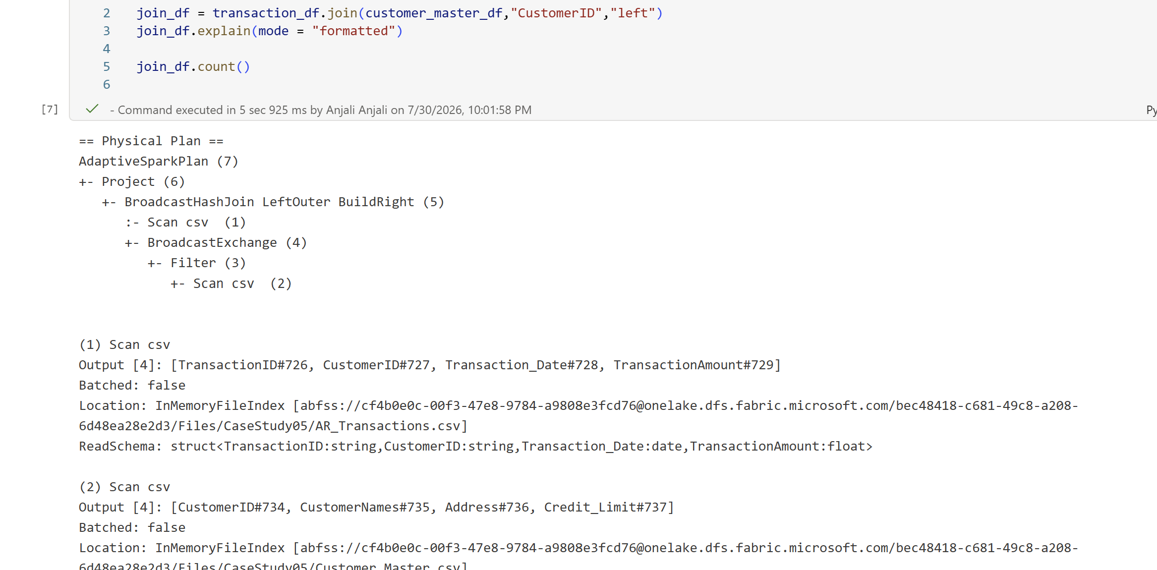
joined_df.explain(mode="formatted")
joined_df.count() View full size (opens in a new tab)
 View full size (opens in a new tab)
Functions used
- spark.conf.set()
- Sets Spark configuration properties during runtime.
- spark.sql.autoBroadcastJoinThreshold
- Specifies the maximum table size that Spark can automatically broadcast during a join.
- join()
- Combines two DataFrames using a common key, here
CustomerID, with a left join. - explain(mode="formatted")
- Displays Spark’s physical execution plan, helping verify the join strategy and identify performance optimisations.
- count()
- Executes the DataFrame transformations and returns the total number of records.
What are we doing? Setting Spark’s broadcast size limit to 10 MB so it automatically
copies small tables across the cluster instead of shuffling all the data, joining the AR
Transactions and Customer Master datasets on the CustomerID column, then checking Spark’s
execution plan to confirm it used the fast broadcast join.
Why are we doing this? The customer master table is much smaller than the AR transactions table. Broadcasting the smaller table to all worker nodes eliminates expensive data shuffling, resulting in faster join execution and better performance. Reviewing the execution plan confirms that Spark is using the most efficient join strategy.
Execution plan highlights
- AdaptiveSparkPlan: Spark dynamically optimises the query execution at runtime.
- BroadcastHashJoin: confirms that Spark selected the optimised broadcast join strategy.
- BroadcastExchange: indicates that the customer master table was broadcast to all executors before performing the join.
- Scan CSV: reads the source CSV files before applying transformations and joins.
Broadcast join is a join optimisation technique where Spark copies the smaller table to all worker nodes and joins it with the larger table locally. This eliminates data shuffling, making the join much faster for large datasets.
Sort merge join is a join strategy where Spark shuffles and sorts both tables based on the join key before merging them. It is commonly used when both tables are large and cannot be broadcast.
In simple terms:
- Broadcast join: best for one small table and one large table, so faster.
- Sort merge join: best for two large tables, so slower because of the sorting and shuffling.
Step 3: Validate schema enforcement in Delta Lake
 View full size (opens in a new tab)
 View full size (opens in a new tab)
 View full size (opens in a new tab)
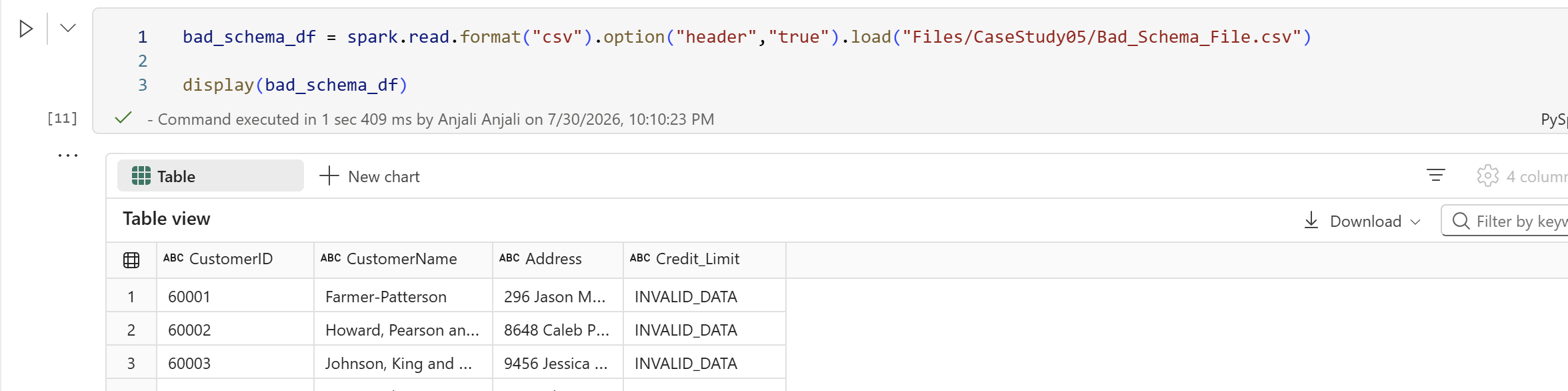
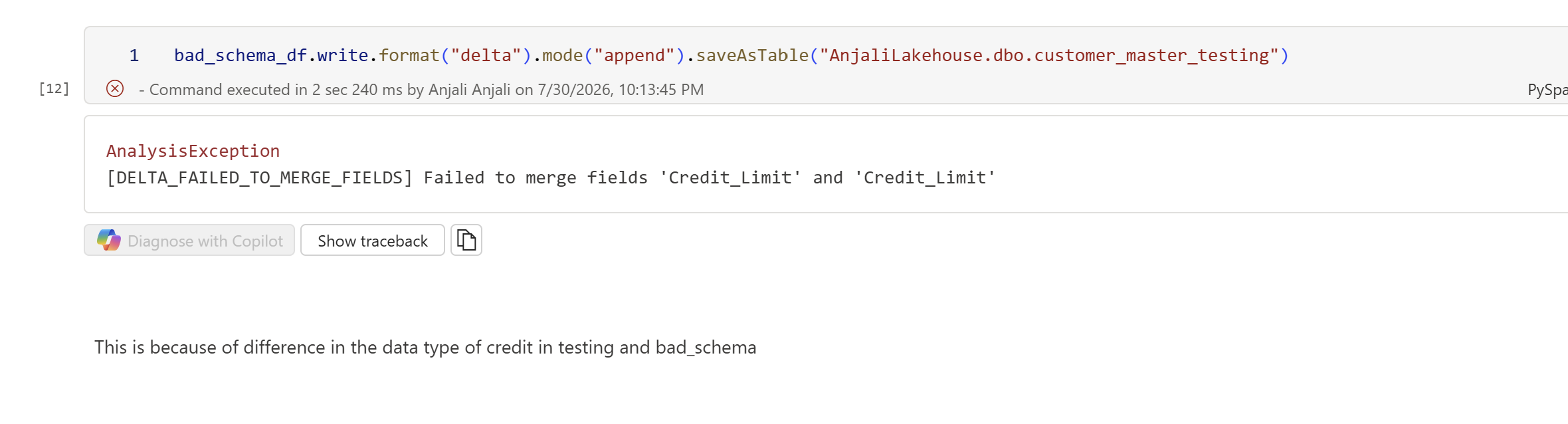
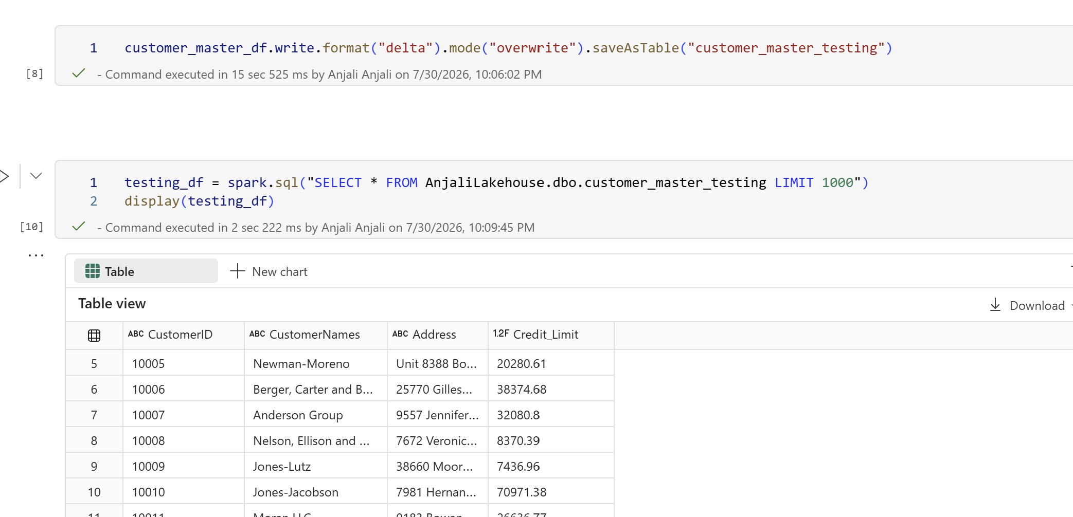
What are we doing? First creating a Delta table from the valid Customer Master dataset,
then loading another dataset with an invalid schema, where the Credit_Limit column has an
incorrect data type, and trying to append it to the Delta table.
Why are we doing this? The objective is to demonstrate Delta Lake’s schema enforcement. Delta Lake validates the schema of incoming data before writing it to the table. If the data types do not match, it rejects the write operation, preventing invalid or inconsistent data from being stored.
Step 4: Time Travel and RESTORE
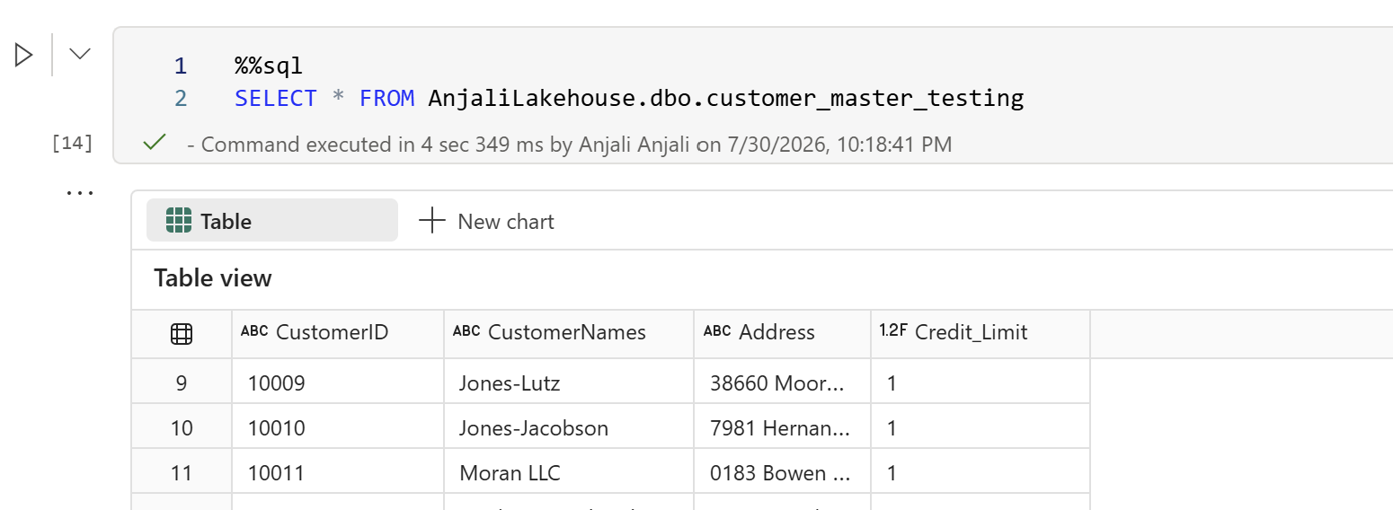
UPDATE customer_master_testing SET Credit_Limit = 1;
SELECT * FROM customer_master_testing;
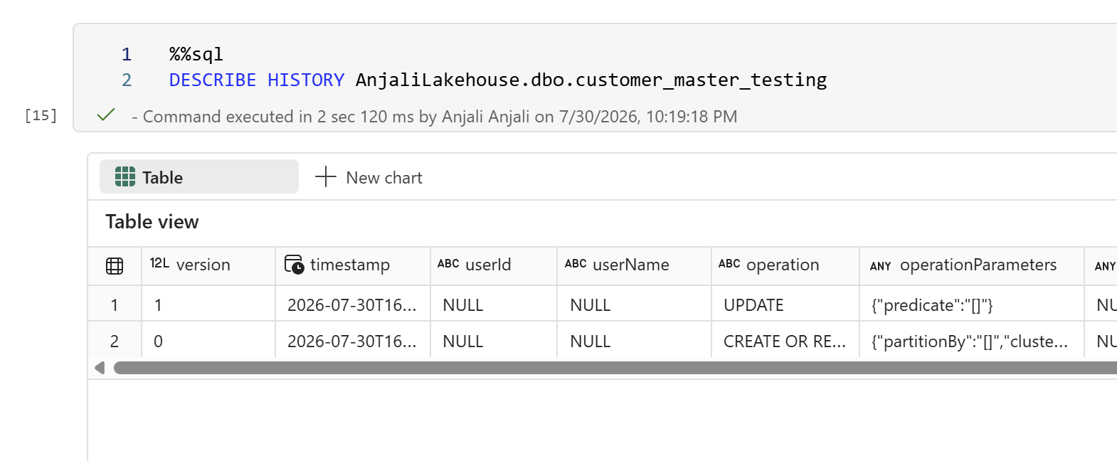
DESCRIBE HISTORY customer_master_testing;
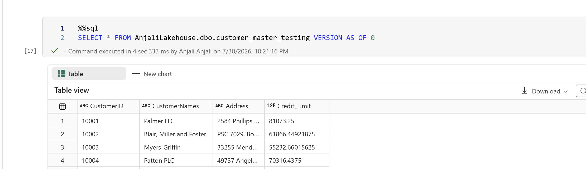
SELECT * FROM customer_master_testing VERSION AS OF 0;
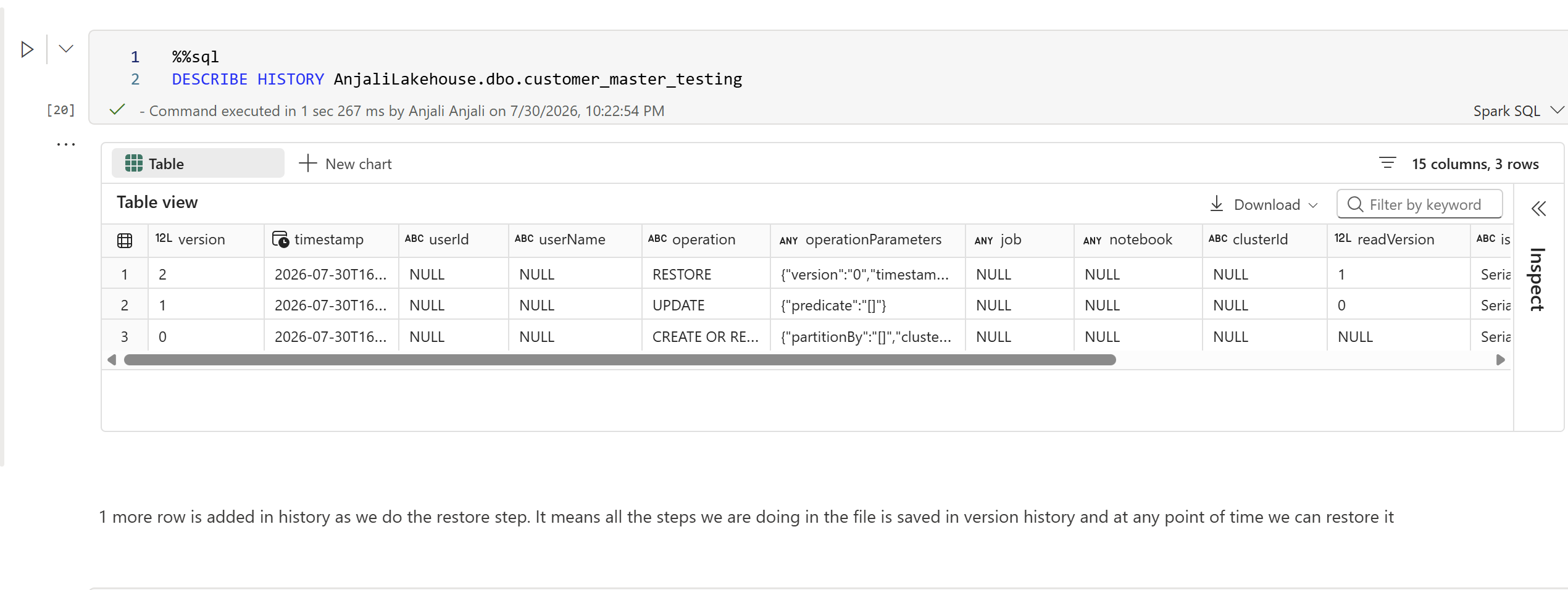
RESTORE TABLE customer_master_testing VERSION AS OF 0;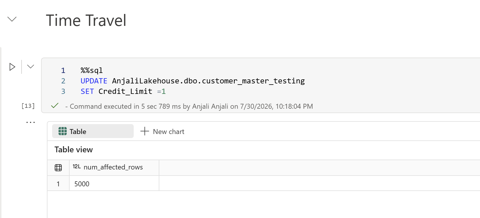 View full size (opens in a new tab)
 View full size (opens in a new tab)
 View full size (opens in a new tab)
 View full size (opens in a new tab)
 View full size (opens in a new tab)
 View full size (opens in a new tab)
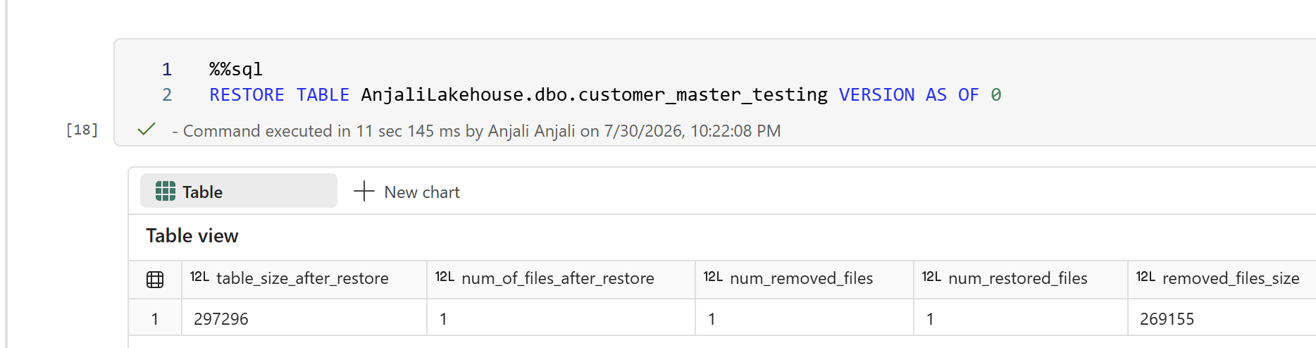
What are we doing? Updating all records in the customer_master_testing Delta table by
setting Credit_Limit to 1. After the update, checking the modified data, viewing the
table’s version history, retrieving the original data using Time Travel, and finally
restoring the table to its previous version.
Why are we doing this? This demonstrates Delta Lake Time Travel, which allows previous versions of a table to be accessed and restored. It helps recover data after accidental updates or deletions, supports auditing, and enables tracking of historical changes without requiring backups.
Functions used
- UPDATE
- Modifies existing records in the Delta table.
- SELECT
- Displays the current contents of the table after the update.
- DESCRIBE HISTORY
- Shows the version history and all operations performed on the Delta table.
- VERSION AS OF
- Reads data from a specific historical version of the table.
- RESTORE TABLE … VERSION AS OF
- Restores the Delta table to a selected previous version.